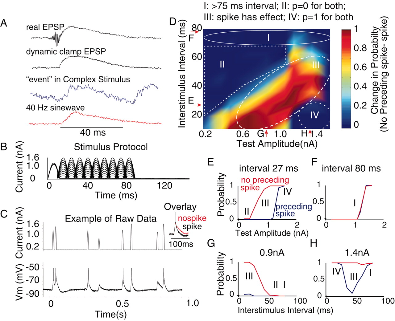
Examination of the reduced probability of spiking after the generation of an action potential in cortical neurons. A, Example waveforms of the response of cortical cells to activation of a real EPSP (from Fig. 1), a dynamic clamp EPSP (from Fig. 2), one of the larger “events” in the complex waveform (from Fig. 9A), and injection of the depolarizing phase only of a 40 Hz sine wave (see B). The peak amplitudes of the waveforms were normalized to the same value to facilitate the comparison of time courses. All of the wave forms are of a similar time course. B, Protocol for examining the effect of spike generation on the responsiveness of the neuron. The depolarizing half of a 40 Hz sine wave was injected, followed at various intervals by injection of the same waveform but at different amplitudes. The first current injection was of two different amplitudes and adjusted so that the larger amplitude caused an action potential, whereas the smaller failed to do so. C, Example of raw data. The amplitude and time of occurrence of the second sine wave were pseudorandomized (between discrete time steps of 9-10 msec). Overlay, Membrane potential response of the cell to the sine wave injection that caused a spike (black) and one that did not cause a spike (red). Note that the occurrence of a spike shortens the falling phase of the response. D, Plot of the change in probability of eliciting an action potential by inputs of various amplitudes and at various intervals after the generation of a spike. The change in probability is calculated by subtracting the probability curve with a spike from the curve without a spike for each amplitude-time point (e.g., see E-H as indicated by arrows). There are four distinct regions. Region I represents a separation of the two stimuli by ≥70 msec. In this region, the occurrence of a spike to the first input has little or no effect on the probability of generating a spike to the second. Region II represents amplitudes and time intervals in which the probability of generating an action potential to either input was 0. Region III represents those amplitude and time intervals in which the occurrence of a spike to the first stimulus significantly reduced the probability of spiking to the second stimulus. In region IV, the test stimulus was so large and at such a short interval that the occurrence of a spike to the first had no effect. E, Example of the spike probability curve for different-amplitude inputs with and without a preceding spike at an interval of 27 msec. F, At an interval of 80 msec, the generation of a spike has no effect. G, Effect for different intervals at a fixed amplitude of the test stimulus. At short intervals, there is significant temporal summation, which is reduced by the occurrence of an action potential. H, Example curves for 1.4 nA input at different intervals. There are two main effects. At short intervals, there is temporal summation, which overcomes the suppressive effect of a preceding spike. At long intervals, the preceding spike has no effect. Between these extremes, the occurrence of a spike reduces the probability of generating another action potential.