Effective Connectivity Reveals an Interconnected Inferotemporal Network for Three-Dimensional Structure Processing
- Laboratory for Neuro- and Psychophysiology, KU Leuven, 3000 Leuven, Belgium; the Leuven Brain Institute, 3000 Leuven, Belgium
-
Author contributions: E.P. and P.J. designed research; E.P. performed research; E.P. contributed unpublished reagents/analytic tools; E.P. analyzed data; E.P. and P.J. wrote the first draft of the paper; E.P. and P.J. edited the paper; E.P. and P.J. wrote the paper.
Abstract
Disparity-defined 3D shape is processed in both the ventral and the dorsal visual stream. The network of cortical areas that is activated during the processing of disparity-defined 3D shape includes, in addition to parietal and premotor areas, three clearly distinct regions in inferotemporal cortex (ITC). To investigate the connectivity of the latter regions, we combined electrical stimulation with fMRI in male macaque monkeys. Electrical stimulation of each of the 3D-structure nodes in ITC mainly elicited increased fMRI activations in the other 3D-structure nodes and more variably in other parts of ventral visual cortex. Importantly, no increased activation was found in parietal areas, nor in PFC, whereas microstimulation in posterior parietal cortex did activate the ITC. Our results indicate that 3D-structure nodes in ITC form a strongly interconnected network, receiving input from parietal areas implicated in 3D-structure processing.
SIGNIFICANCE STATEMENT Previous studies combining electrical microstimulation with functional imaging showed an interconnected set of regions in the ventral stream processing faces or bodies, but is has been unclear whether the same is true for other visual categories. Here the authors show that there is a connected system of stereo-selective regions in inferotemporal cortex, receiving input from parietal areas in the dorsal stream.
Introduction
Previous single-cell (Janssen et al., 1999, 2000a,b; Yamane et al., 2008; Srivastava et al., 2009; Verhoef et al., 2011) and monkey fMRI studies (Durand et al., 2007; Joly et al., 2009) have shown that disparity-defined 3D shape is processed in both the ventral (inferior temporal cortex [ITC]) and the dorsal visual stream. In the ventral stream, most single-cell studies have targeted a region in the lower bank of the rostral superior temporal sulcus (STS, area TEs), where neurons selective for disparity-defined 3D shape are concentrated (Janssen et al., 2000a). Electrical microstimulation (EM) of clusters of 3D-shape selective neurons in TEs predictably alters the perceptual choice of rhesus monkeys that are categorizing 3D structure from disparity (Verhoef et al., 2012): monkeys are more likely to choose “convex” when weak electrical stimulation is applied in a convex-preferring cluster of neurons in TEs during the decision process. Furthermore, reaction times are shorter when the animal chooses the choice target corresponding to the preference of the stimulated site, and slower when choosing the alternative choice target. These results indicate that neural activity in TEs is causally related to the categorization of 3D structure (convex or concave).
The network of cortical areas that is activated more by curved surfaces than by flat surfaces at different disparities includes parietal areas (caudal intraparietal area [CIP], posterior intraparietal area [PIP], and the anterior parietal area [AIP]); premotor area F5a, and three clearly distinct (sub)sectors in the ventral stream: posterior inferotemporal area (TEO); a region in posterior TE on the convexity (TEp); and a more anterior STS region (TEs) (Van Dromme et al., 2016). Recently, we have charted the effective connectivity of the dorsal stream 3D shape-selective sites using a combination of single-cell recordings, EM, reversible inactivation, and fMRI (Premereur et al., 2015; Van Dromme et al., 2016). Microstimulation of anterior AIP activates a somatomotor network comprising the rostral part of the inferior parietal lobule; the medial intraparietal area; the secondary somatosensory cortex; and ventral premotor cortex (F5), whereas microstimulation of posterior AIP activates areas involved in object processing, including CIP, TEO, and TE. Furthermore, reversible inactivation of area CIP causes significant reductions in 3D-structure-related fMRI activations in areas AIP and in area TE (Van Dromme et al., 2016). Thus, investigating the connectivity of area AIP provided crucial data about the information flow from visual areas, through AIP, to somatomotor areas involved in object grasping. Importantly, EM of area CIP did not elicit increased fMRI activation in ITC or AIP, indicating that CIP executes its influence on the end-stage areas of the dorsal and ventral stream indirectly, through another parietal area (ventral intraparietal area or dorsal lateral intraparietal area).
To date, it remains unclear how 3D structure information flows through the ventral stream, and which are the target areas of the ventral stream 3D-structure nodes outside the temporal lobe. In the current project, we investigated the effective connectivity in the ventral stream 3D-structure nodes by means of EM during fMRI.
Materials and Methods
All experimental procedures were performed in accordance with the National Institutes of Health Guide for the care and use of laboratory animals and EU Directive 2010/63/EU, and approved by the Ethical Committee on Animal Experiments at the KU Leuven. The animals used in this study (4 adult male rhesus monkeys) were housed in accordance with the recommendations of the Weatherall report, allowing locomotor behavior, social interactions, and foraging. All animals were pair- or group-housed (2-4 animals per group; cage size at least 16-32 m3) with cage enrichment (toys, foraging devices) at the primate facility of the KU Leuven Medical School. They were daily fed with standard primate chow supplemented with bread, nuts, raisins, prunes, and fruits. All animals had a custom-made, MRI, compatible headpost and recording chamber implanted on the skull using ceramic screws and dental acrylic. All surgeries were performed under isoflurane or propofol anesthesia and sterile conditions. The animals received their daily water supply either during the awake fMRI experiments, or ad libitum in the cages before and after sedated (fMRI) experiments.
Scanning
Functional images were acquired with a 3.0 T full-body scanner (Magnetom Trio and Prisma; Siemens), using a gradient-echo T2*-weighted EPI sequence (40 horizontal slices; TR: 2s; TE: 16 ms; 1.25 mm3 isotropic voxels) with a custom-built 8-channel phased-array receive coil, and a saddle-shaped, radial transmit-only surface coil (Ekstrom et al., 2008). Before each scanning session, a contrast agent, monocrystalline iron oxide nanoparticle (Feraheme: AMAG Pharmaceuticals), was injected into the femoral/saphenous vein (7-11 mg/kg) (Vanduffel et al., 2001). An MPRAGE sequence (144 horizontal slices; 0.6 mm3 isotropic voxels) was acquired in the beginning of every EM-fMRI session to verify the electrode location (TR: 2700 ms; TE: 3.8 ms; TI: 850 ms; flip angle: 90).
Experimental design and statistical analysis
fMRI localizer experiments
fMRI localizer experiments were performed as described previously (Van Dromme et al., 2016). After adequate performance in passive fixation had been reached, the animals were trained in a depth structure categorization task (concave-convex discrimination by means of an eye movement) to verify their stereo vision. All animals performed >80% correct. The fMRI localizer data were obtained during passive fixation in an electronically defined 2 × 2 degree window. During all fMRI experiments, the animals were seated in sphinx position (Vanduffel et al., 2001) in a plastic monkey chair directly facing an LCD screen (viewing distance: 57 cm). Eye position was monitored at 120 Hz through the pupil position (Iscan).
The stimulus set consisted of curved and flat random-dot stereograms in which depth was defined by horizontal disparity (dot size 0.08 deg, dot density 50%, vertical size 5.5 deg), presented on a gray background. All stimuli were generated using MATLAB (R2010a, The MathWorks) and were γ-corrected. Similar to previous studies (Durand et al., 2007; Joly et al., 2009; Van Dromme et al., 2016), we used a 2 × 2 design (see Fig. 1A) with factors curvature (curved vs flat) and disparity (stereo vs control, in which the control condition consisted of the monocular images of the stereo condition presented to the two eyes simultaneously). The curved-stereo condition consisted of three types of smoothly curved depth profiles (1, one-half, or one-fourth vertical sinusoidal cycle) together with their antiphase counterparts obtained by interchanging the monocular images of the two eyes (disparity amplitude within the surface: 0.5°). Four different circumference shapes were combined with each of these six depth profiles, and each combination could appear at two different positions in depth (mean disparity ±0.5°), creating a set of 48 curved surfaces. In the flat-stereo condition, flat surfaces (using the same four circumference shapes) were presented at 12 different positions in depth, such that the average disparity content was identical to that in the curved stereo condition. Finally, in the control conditions, we presented one of the monocular images (either belonging to one of the curved stereo stimuli of to one of the flat stereo stimuli) to both eyes simultaneously (curved-control and flat-control). These control conditions consisted of the same binocular input as the stereo conditions, since they contained exactly the same monocular images as the corresponding stereo condition. Red/green stereoglasses were placed before the eyes to provide dichoptic presentations of the stimuli. Maintenance of fixation around the fixation point was required to be rewarded. Using this stimulus set, a large number of single-cell studies have confirmed the validity of the fMRI localizer in TEs, AIP, F5a, PIP, CIP, and TEO (Verhoef et al., 2012; Theys et al., 2013; Alizadeh et al., 2018a,b). The inter-reward interval was systematically decreased (from 2000 to 900 ms) when the monkey maintained fixation within the window, to encourage long, uninterrupted sequences of fixation.
Data were acquired using a block design whereby each condition (24 s long) consisted of 12 functional volumes embedded in a time series of 222 volumes (444 s). Each condition (or block) was repeated twice within each time series. The presentation order of the conditions was pseudo-randomized. Stimulus presentation frequency was 1 Hz. Voxels showing a significant interaction between the factors curvature and disparity, that is, where (curved stereo vs curved control) was greater than (flat stereo vs flat control), were deemed to be sensitive to the depth structure of surfaces.
EM combined with fMRI
All procedures were as previously described (Premereur et al., 2015, 2016; Van Dromme et al., 2016). Briefly, during combined EM-fMRI experiments, the animals were sedated using a 33%/66% mixture of ketamine (Nimatek; Eurovet; 12.5 mg/30 min) and medetomidine (Domitor; Orion; 0.25 mg/30 min). We have previously demonstrated highly similar results in awake versus sedated animals (Premereur et al., 2015). Previous studies (Moeller et al., 2008; Premereur et al., 2013) have indicated an effect of the task the animal was performing on the EM-induced activations. EM during less cognitively demanding tasks evoked results more similar to the known anatomic connectivity patterns, while EM during more demanding tasks even elicited activations in second synapses. To ensure that our results mimic the anatomic connectivity as closely as possible, we performed the experiment on sedated animals.
In every scanning session, a platinum/iridium electrode (impedance 50-200 kΩ in situ, FHC) was inserted in the grid through glass capillaries (0.5 mm inner diameter) serving as guide tubes (FHC). The electrodes were lowered in a grid position and to a depth corresponding to the center of the fMRI activations as defined by the stereo-localizer. To verify the electrode locations, structural MR images (0.6 mm isotropic resolution) were acquired in every scan session (before the start of the fMRI experiment) while the electrode was located at the stimulation site. During the microstimulation experiment, a platinum wire (BASi) inserted in the grid and touching the dura, served as ground. The EM signal was produced using an 8-channel digital stimulator (DS8000, World Precision Instruments) in combination with a current isolator (DLS100, World Precision Instruments). We alternated between no-stimulation and stimulation blocks (each lasting 40 s), with each run lasting 245 NMR-pulses (490 s). During stimulation blocks, 250 ms EM trains were applied, with a random time between two consecutive EM trains (on average 2099 ms; range: 1986-2232 ms). Stimulation trains were composed of biphasic square-wave pulses (frequency: 200 Hz, amplitude: 1 mA). Each pulse consisted of 190 μs of positive and 190 μs of negative voltage, with 0.1 ms between the two pulses (total pulse duration: 0.48 ms) (Ekstrom et al., 2008; Premereur et al., 2013). The timing of the EM pulses during the fMRI experiment was computer-controlled (Premereur et al., 2015). The current amplitude of 1 mA was determined based on previous studies (Premereur et al., 2015, 2016; Van Dromme et al., 2016), in which we observed that a current strength of 1 mA evoked the most reliable EM-induced activations.
fMRI data analysis
For the stereo-localizer experiment, offline image reconstruction was conducted to overcome problems inherent to monkey body motion at 3T (Kolster et al., 2009). Both the localizer and EM experiments were analyzed using statistical parametric mapping (SPM5, SPM12) and BrainMatch software, using a fixed-effects GLM. Realignment parameters were included as covariates of no interest to remove brain motion artifacts. Spatial preprocessing consisted of realignment and rigid coregistration with the animal's own anatomic scan. The functional volumes were then resliced to 1 mm3 isotropic and smoothed with an isotropic Gaussian kernel (FWHM: 1.5 mm).
Single-subject analyses were performed, and the level of significance was set at p < 0.001, uncorrected for multiple comparisons. Importantly, the exact locations and extents of the EM-induced fMRI activations were verified on the animal's own EPI images.
Percent signal change (PSC) was calculated using MarsBaR (version 0.44) and averaged over runs. Standard error of the mean (SEM) was calculated over runs. Significant changes in PSC compared with the no-EM condition (no-EM condition is set as the baseline with a PSC of 0) were calculated using t tests, Bonferroni-corrected for the number of (sub)sectors.
We also calculated the PSCs in 12 visual areas in the ipsilateral (i.e., the stimulated) hemisphere based on the probabilistic maps described previously (Janssens et al., 2014). Because the exact boundaries between these areas are often difficult to determine, we grouped these 12 visual areas into four clusters: the V1-V2-V3 cluster, the V4 cluster (comprising V4, V4A, and V4t), the PIT cluster (comprising OT, PITd, and PITv), and the MT/MST/FST cluster.
Results
The fMRI stereo-localizer experiment was performed in 4 animals (Monkey S: 79 runs, Monkey A: 57 runs, Monkey M: 55 runs; Monkey K: 72 runs; Fig. 1B,C). To obtain an overview of the cortical network that is sensitive to depth structure, t values were calculated for the contrast [(curved stereo vs curved control) – (flat stereo vs flat control)] (stimuli in Fig. 1A). In accordance with previous results (Van Dromme et al., 2016), we found significant fMRI activations in parietal areas (dLIP, ventral intraparietal area, PIP, CIP, AIP), in premotor and prefrontal areas (45, F5a, data not shown), in somatosensory area secondary somatosensory cortex (data not shown), and in at least three clearly separated patches in ITC. The most posterior ITC activation was located in area TEO on the lip of the STS (Fig. 1B,C), the middle patch was located in the posterior part of area TE on the temporal convexity (TEp, Fig. 1B,C), and the most anterior patch appeared in the lower bank and lip of the STS in the anterior part of area TE (TEs). The latter TEs activation spanned several millimeters in the anterior-posterior direction, at the level of the hippocampus and amygdala (Fig. 1C, bottom panels). Although we could detect at least one stereo-defined hotspot in TEs in every animal tested, we often observed two clearly separated hotspots in the rostral STS (Monkey S: right hemisphere, Monkey K, both hemispheres, indicated with two blue arrows). To date, no behavioral implications of the presence of two TEs hotspots have been described, and all animals used in this study had excellent stereovision as tested in a stereo-discrimination task. In the remainder of the manuscript, we will combine all voxels of these two hotspots and refer to this combination as TEs. The most posterior hotspot was stimulated in case two TEs hotspots were present. Only Monkey A showed an additional more anterior and ventral stereo-defined patch along the anterior middle temporal sulcus (AMTS) (Fig. 1B,C, red arrow). The effective connectivity of the stereo-defined ITC patches in TEs, TEp, and TEO, which were present in all animals, was tested in at least 2 of the animals by combining EM with fMRI (EM-fMRI) (Table 1).
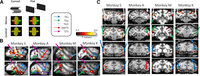
3D structure processing network. A, Stimuli. A 2 × 2 design was used with factors curvature (curved vs flat) and disparity (control vs stereo). B, t values for the contrast [(curved stereo – controls) – (flat stereo-controls)] are displayed for 4 animals (p < 0.001, uncorrected) in two sagittal sections per subject. Arrows indicate inferotemporal hotspots: blue arrow indicates TEs; green arrow indicates TEp; white arrow indicates TEO; red arrow indicates AMTS. C, Coronal sections for individual subjects.
Overview of the number of EM-sessions per subject (Monkeys S, K, A, and M) and stimulated stereo-defined ITC patcha
Area TEs
We lowered stimulation electrodes toward the hotspot of the stereo activations in the most anterior stereo-defined IT patch, TEs. The location of the electrode tip was verified with respect to the activations induced by the stereo-localizer experiment as in Figure 1 (see Fig. 2A). Both animals showed two TEs hotspots; and for both subjects, the most posterior one was stimulated. To investigate the effective connectivity of TEs, we applied EM during fMRI in 2 animals (for overview of the number of sessions, see Table 1) and found TEs-EM to induce robust fMRI activations in the two other stereo-defined patches in ITC: TEO (Fig. 2B–D, white arrows) and TEp (Fig. 2B–D, green arrows), but not in parietal or prefrontal/premotor areas (Fig. 2C). Indeed, for both animals, TEs-EM induced increased activations in clearly distinct sectors along the inferotemporal sulcus, which corresponded with the stereo-activations (Fig. 2B,D, compare EM activations with white outlines indicating stereo-localizer). TEs-EM also elicited a very small activation around the AMTS for Monkey K (Fig. 2D, red arrow), while the AMTS was however not activated during the stereo-localizer for the latter animal.

TEs microstimulation. A, t values for the contrast [(curved stereo – controls) – (flat stereo-controls)] are displayed for 2 animals (Monkeys K and S) on their own anatomic scan (p < 0.001, uncorrected). Black artifact indicates the position of the stimulation electrode (indicated with blue arrows). B, Top row represents t values for the 3D processing network. Bottom row represents t values for the contrast (TEs microstimulation vs no microstimulation). t values are plotted for the 2 subjects individually. The same sagittal slice is displayed for each animal in the top and bottom row. C, Top row represents t values for the 3D processing network. Bottom row represents t values for the contrast (TEs microstimulation vs no microstimulation). Focus on parietal, premotor, and prefrontal areas. All conventions are as in B. D, t values for the contrast (TEs microstimulation vs no microstimulation; p < 0.001, uncorrected). t values are plotted for the 2 animals individually. White outlines indicate the outline of the activations of the 3D processing network as in Figure 1. Distance between two coronal slices is 2 mm. Anteroposterior coordinate of the center slice is indicated with 0. Arrows indicate the inferotemporal stereo hotspots as in Figure 1. Dashed blue arrow indicates TEs-EM induced activations outside the stereo-localizer.
Consistent with the increased fMRI activity in stereo-defined patches TEO and TEp during TEs-EM, TEs-EM also significantly increased the PSC (compared with the no-EM baseline) in TEp and TEO (Fig. 3A; t tests, p < 0.05, Bonferroni-corrected for multiple comparisons; for statistical tests, see Table 2). TEs-EM significantly activated (p < 0.001, uncorrected) 3%–75% of the voxels of the stereo-defined IT patches TEO and TEp (Table 3).

TEs-EM. A, PSC during TEs microstimulation. **Significant increases compared with baseline (t tests, Bonferroni-corrected, p < 0.05). Error bars indicate SEM over runs. Lightning symbols indicate stimulated area. B, Comparing TEs-EM and pAIP-EM in the same animal. Same coronal and sagittal sections are shown for pAIP-EM and TEs-EM. White arrow indicates TEO. Blue arrow indicates TEs.
t values for increases in PSC (compared with no-EM baseline) in stereo-defined IT patches for the stimulated areas per subject
Percent voxels of stereo-defined ITC patches TEs, TEp, and TEO significantly (p < 0.001) driven by EM of other ITC patches for all individual subjects (Monkeys S, K, A, and M) and hemispheresa
A small number of TEs-EM-activated voxels were located outside of the stereo-localizer (example in Fig. 2D, top row: Monkey K; EM-induced activations extend more anterior to stereo-defined TEs, indicated with dashed blue arrow). Importantly, though, part of the EM-activated voxels outside the stereo-localizer were also activated during the mere presentation of visual stimuli (contrast [all stimuli − fixation], p < 0.001, uncorrected; in Monkey K, 36% of EM-driven voxels outside the stereo-localizer were significantly visually driven, in Monkey S: 13%). TEs-EM did not evoke any significant contralateral activations (Fig. 2D).
The results described above suggest that TEs is connected primarily to the other patches of the 3D structure network and to other visually driven voxels in the ITC. Surprisingly, EM of area TEs did not elicit fMRI activations in stereo-defined areas in parietal, somatosensory, or premotor cortex, nor in any other part of parietal or frontal cortex (Fig. 2C,D), although EM in posterior AIP (pAIP) does activate TEs (Premereur et al., 2015). Even within the same animal (Monkey K, data from Premereur et al., 2015), microstimulation of pAIP (the posterior hotspot of stereo-defined AIP) significantly activated TEs (Fig. 3B, blue arrow, top row; p < 0.001, uncorrected; PSC in Table 4), but TEs-EM did not induce activations in any part of AIP (Fig. 3B, bottom row; t values shown for the contrast [EM vs no-EM], p < 0.001, uncorrected; PSC calculated in stereo-defined AIP: Table 4).
ITC-EM and pAIP-EMa
We also examined to what extent TEs-EM activated other visual areas that are not part of the 3D-structure network. Figure 4A shows the PSCs in 12 visual areas in the ipsilateral (i.e., the stimulated) hemisphere based on the probabilistic maps described by Janssens et al. (2014). We grouped the areas in four clusters (Fig. 4, colored boxes), and mainly found increased TEs-EM-induced activations in the PIT cluster. For Monkey K, TEs-EM elicited also increased activations in OT, PITv, V4A, V4, and V4t of the same hemisphere, and a significant deactivation in V1. However, for unknown reasons, the latter activations were not replicated in Monkey S (t values in Table 5).

PSC. A, TEs-EM induced PSC in 12 different regions of interest (ROIs) for individual subjects, indicated with different shades of gray. Only ROIs in the hemisphere ipsilateral to the stimulation site are included. Bar plot represents average PSC per subject over runs. Error bars indicate SEM over runs. Significance was tested with a t test. **p < 0.05 (Bonferroni-corrected for number of comparisons). *p < 0.05 (not corrected). B, TEp-EM induced PSC. C, TEO-EM induced PSC. Colored squares represent clusters of neighboring areas: red square represents MT/MSTv/MT cluster; green square represents PIT cluster; yellow square represents V1-V2-V3 cluster; blue square represents V4 cluster.
t values for increases in PSC (compared with no-EM baseline) in ROIs for the stimulated areas per subject
Area TEp
Similar to TEs, we performed EM-fMRI in stereo-defined TEp in 2 animals, in three hemispheres (for electrode localization, see Table 1; Fig. 5A). EM in TEp activated (at p < 0.001, uncorrected) stereo-defined TEs and TEO (Fig. 5B–D) in at least 25% of the voxels in the latter patches (except for TEs in Monkey A: Table 3), while no activation was induced in parietal or prefrontal areas (Fig. 5C). TEp-EM significantly increased the PSC (compared with the no-EM baseline) in stereo-defined patches in TEO and TEs (Fig. 6; t tests, p < 0.05, Bonferroni-corrected for multiple comparisons, statistics in Table 2). The EM-induced PSCs measured in TEO and TEs were relatively similar in both monkeys (except the right hemisphere in Monkey S). Importantly and similar to our TEs-EM experiments, EM of area TEp did not elicit increased activations in parietal, somatosensory, or premotor cortex (Fig. 5C), nor in TEp of the contralateral hemisphere. Similar to TEs-EM, TEp-EM also activated voxels outside the stereo-localizer (e.g., Fig. 5D, dashed white arrow for Monkey A), but a large part of these voxels were also activated during the mere visual presentation of stimuli (Monkey Sleft: 40% of EM-driven voxels outside stereo-localizer were significantly visually driven; Monkey Sright: 44%; Monkey A: 70%). These activations were located in both areas TE and TEO (Fig. 5D, dashed arrows). Outside the stereo-localizer, the EM-induced activations were more variable (Fig. 4B). However, in all three TEp-EM-experiments, we found a significant TEp-induced increase in PSC in ventral stream areas OT, PITd, and in at least one of the areas of the V4 cluster (V4, V4A, and V4t, t tests corrected for number of comparisons, p < 0.05; for statistics, see Table 5). In contrast, we rarely observed significant activations in the MT/MST/FST cluster after TEp stimulation (Fig. 4B).

TEp microstimulation. A, t values for the contrast [(curved stereo – controls) – (flat stereo-controls)] are displayed for 2 animals (Monkey S in both hemispheres; p < 0.001, uncorrected). Electrode artifact is shown in the anatomic scan (indicated with green arrows) for three hemispheres (SRight, SLeft, and K). B, Top row represents t values for the 3D processing network. Bottom row represents t values for the contrast (TEp-EM vs no EM). C, Top row represents t values for the 3D processing network. Bottom row represents t values for the contrast (TEp-EM vs no EM). D, t values for the contrast (TEp-EM vs no EM; p < 0.001, uncorrected). White outlines indicate the outline of the activations of the 3D processing network as in Figure 1. Arrows indicate the inferotemporal hotspots as in Figure 1. All conventions are as in Figure 2.

PSC during TEp microstimulation. **Significant increases compared with no-EM baseline (t tests, Bonferroni-corrected, p < 0.05). Error bars indicate SEM over runs. Lightning symbols indicate stimulated area.
Area TEO
Finally, we applied EM during fMRI in stereo-defined TEO in 3 animals (for electrode localization, see Table 1; Fig. 7A). EM in TEO elicited increased fMRI activations in distinct patches along the ITC (Fig. 7B–D), but not in parietal or prefrontal/premotor areas (Fig. 7C,D). Indeed, TEO-EM-induced activations in stereo-defined TEp (Fig. 7D, green arrow) and TEs (Fig. 6D, blue arrows), and significantly increased the PSC in these areas (compared with no-stimulation baseline, t tests, p < 0.05, Bonferroni-corrected for multiple comparisons, except for TEp in Monkey K; Fig. 8, Table 2 for statistics). The lack of activation in TEp in Monkey K is most likely because of small deformations of the brain (because of the implantation of the cylinder, which causes growth of inflammatory tissue resulting in slight deformations of the underlying cortex), as voxels dorsal to TEp did show significant EM-induced increase. Furthermore, TEO-EM elicited significant fMRI activations (p < 0.001, uncorrected) in 14%–61% of the voxels in stereo-defined TEp and TEs (except TEp in Monkey K; Table 3). Figure 7D also shows that TEO-EM-induced activations were mainly located inside the stereo-defined IT patches. However, a small number of TEO-EM activated voxels were located outside of the stereo-localizer in TEO and TE (example in Fig. 7D, indicated with dashed white arrow for TEO and dashed blue arrow for TE). As in the other ITC patches, part of the EM-activated voxels outside the stereo-localizer were activated during the mere presentation of visual stimuli (Monkey S: 44% of EM-driven voxels outside stereo-localizer are significantly visually driven; Monkey M: 57%; Monkey K: 32%). Similar to the TEs and TEp experiments, the activations induced by TEO-EM outside the stereo-localizer were more variable (Fig. 4C). In all 3 animals, we found EM-induced increased PSC in the V4 and PIT clusters, and very weak activations in the MT/MST/FST cluster (Fig. 4C; t test, p < 0.05, for statistics, see Table 5).

TEO microstimulation. A, t values for the contrast [(curved stereo – controls) – (flat stereo – controls)] are displayed for 3 animals (p < 0.001, uncorrected). Electrode artifacts are shown in the anatomic scan (indicated with white arrows) for all 3 subjects (Monkeys S, M, and K). B, Top row represents t values for the 3D processing network. Bottom row represents t values for the contrast (TEO-EM vs no EM). C, Top row represents t values for the 3D processing network. Bottom row represents t values for the contrast (TEO-EM vs no EM). D, t values for the contrast (TEO-EM vs no EM; p < 0.001, uncorrected). White outlines indicate the outline of the activations of the 3D processing network as in Figure 1. Arrows indicate the stereo-defined inferotemporal hotspots as in Figure 1. Dashed white arrow indicates EM-induced activation outside the stereo-localizer. Conventions as in Figure 2.

PSC during TEO microstimulation. **Significant increases compared with baseline (t tests, Bonferroni-corrected, p < 0.05). Error bars indicate SEM over runs. Lightning symbols indicate stimulated area.
EM of area TEO did not elicit increased activations in parietal, occipital, or frontal cortex (Fig. 7C,D), despite the fact that EM in posterior AIP activates TEO (Premereur et al., 2015). Even within the same animals (Monkey K, Monkey M; data from Premereur et al., 2015), pAIP-EM activated stereo-defined TEO (Fig. 9, top row; p < 0.001, uncorrected) and significantly increased the PSC in the latter area (Table 4), while TEO-EM did not activate any part of AIP (Fig. 9, bottom row; p < 0.001, uncorrected) nor elicited significant increased PSC in AIP (Table 4). pAIP-EM induced activations in TEO both ipsilateral and contralateral to the stimulation site, while TEO-EM did not evoke any contralateral activations.

Comparison of pAIP microstimulation and TEO microstimulation in the same animals. Top row represents t values for the contrast pAIP-EM versus no-EM (p < 0.001, uncorrected) for 2 subjects (one coronal and one sagittal section per subject). Bottom row represents t values for the contrast TEO-EM versus no-EM (p < 0.001, uncorrected) for the same subjects on the same coronal and sagittal section as top row.
Discussion
We charted the effective connectivity of three 3D-structure patches in the macaque ITC (TEO, TEp, and TEs) using EM-fMRI. Our results indicate that the three patches are highly interconnected, but are also connected to other visually driven parts of the ITC outside the stereo patches. However, we could not activate any area in parietal or PFC from any of the stereo patches.
Our results are compatible with the known anatomic connectivity of the ITC (Saleem et al., 2000). Seltzer and Pandya (1978) already described projections from TEO to posterior TE (TE3 in their study) and then to TEs in the lower bank of the rostral STS, as well as direct projections of TEO to TEs and feedback projections from TEs to TEO. The effective connectivity of the 3D-structure patches in the ITC also resembles that of the face and body patch networks (Moeller et al., 2008; Premereur et al., 2016). In both networks, the intrinsic connectivity between the patches appears much stronger than the connectivity with the rest of the brain. It is not surprising that we could also activate other visually driven voxels in the ITC not part of the 3D structure network since 3D structure is merely one of the features of an object, and integration of visual information with respect to 2D shape, texture, and color is necessary for efficient object processing. It is noteworthy that most 3D-structure selective neurons in TEs are also highly selective for the 2D contour of the shape (Janssen et al., 1999). Because of the lack of a generally accepted anatomic and functional subdivision of the ITC, we preferred to not specify in detail which parts of the ITC these EM-activated voxels were located in.
We also activated other visual areas, mainly belonging to the ventral visual stream (OT, PITd, PITv, V4, V4a, and V4t), but rarely dorsal stream areas, such as MT or MST. Moreover, it is clear that at least some of these EM-activated areas partially overlapped with our stereo nodes (e.g., the TEO stereo node and OT/PITd). The activations we induced in V4 were also partially located within the 3D-structure-related activation that we observed in V4. Long-range feedback connections from the most anterior part of TE to intermediate and early visual areas have been described in anatomic tracer studies (Rockland and Van Hoesen, 1994; Saleem et al., 2000).
Similar to previous studies (Moeller et al., 2008; Petkov et al., 2015), our results show variability between monkeys in the strength of the EM-induced activations. The nature of this variability is unclear and could be because of statistical thresholding, differences in signal-to-noise and technical improvements related to the scanner since the data were acquired over several years. It is however more likely that the strongest connected areas show less variability in the EM-induced activations (Moeller et al., 2008). The latter is also visible in our results and supports our main finding observed in all subjects; that is, that the ITC nodes involved in processing 3D structure can be activated by EM but not the parietal nodes of the network. We do not claim that our EM-fMRI approach allowed distinguishing neighboring areas (e.g., V4A, V4, and V4t) that do not belong to the stereo network. Therefore, we preferred to describe the activations outside the stereo-localizer in clusters of areas (the V4, the PIT, and the MT/MST/FST clusters). With this approach, we observed a more consistent pattern of results across animals, that is, reliable activations in the V4 and PIT clusters, and weak or absent activations in the MT/MST/FST and V1-V2-V3 clusters, with the exception of the TEs results.
In addition to variability in the EM results, we also observed variability in the stereo-defined patches in ITC, with some animals showing two TEs patches and others only one. All animals had excellent stereo vision, so it is not possible to relate the TEs activations to behavioral performance. The stereo-localizer scans were obtained in the different animals over a period of several years, and we observed that mainly the temporal activations improved substantially because of technical developments (the 8-channel coil). For example, Monkey M had a very weak unilateral TEs activation in the first localizer scans, but much larger and bilateral TEs activations in the study of Van Dromme et al. (2016). It is well known that the more anterior temporal areas suffer from a loss in signal-to-noise ratio, and this has been improved by the coil design. To minimize the effect of the between-subject variability in the number of TEs activations (one or two), we chose to always stimulate the most posterior activation, which was present in every hemisphere. With these precautions, we consistently activated both TEp and TEO in 2 animals, although for unknown reasons the EM-induced activations outside the stereo patches were markedly more variable (e.g., V4 activations in one animal but not in the other).
Clarifying the effective connectivity of the 3D-structure patches in the ITC is highly relevant for a comprehensive theory on how the primate brain computes the 3D structure of objects from disparity. At the input stage of the ITC network, in area TEO, neurons respond stronger to curved surfaces than to flat surfaces, but no clear selectivity for the sign of curvature (concave or convex) exists (Alizadeh et al., 2018a). The most anterior 3D-structure patch in TEs, in contrast, contains a very detailed representation of depth structure (Janssen et al., 2000b), with an exquisite sensitivity to very small differences in curvedness (Janssen et al., 2000a), which is tightly linked to 3D-structure perception (Janssen et al., 2003; Verhoef et al., 2010, 2012). At present, no single-cell data are available on the middle 3D-structure patch in TEp. In parallel with the ITC network, the dorsal stream builds another representation of 3D structure that evolves from almost exclusively first-order in PIP (Alizadeh et al., 2018b) and most likely in CIP (Tsutsui et al., 2002; Rosenberg and Angelaki, 2014) to second-order in AIP (Srivastava et al., 2009; Van Dromme et al., 2015). Moreover, the posterior subsector of AIP is connected to the ITC (Premereur et al., 2015). A final piece of evidence came from reversible inactivation of area CIP during fMRI (Van Dromme et al., 2016): inhibiting CIP reduced the 3D-structure activations in AIP and TEs, but not those in TEO. In the current study, we demonstrated that the three 3D-structure sensitive patches in the ITC form a highly interconnected network, from which we could not elicit any parietal or prefrontal activation. It appears therefore that, despite the existence of bidirectional connections between AIP and the ITC (Borra et al., 2008), the parietal input to the ITC is much stronger than in the opposite direction, which is consistent with a very large body of anatomic and electrophysiological evidence (for review, see Janssen et al., 2018).
In the light of our findings, it is also interesting to compare the effects of EM in AIP and TEs on behavior. TEs-EM induced strong and predictable effects on perceptual choice in a 3D structure categorization task, including faster reaction times when the animals chose the preferred 3D structure of the stimulation site (Verhoef et al., 2012). In contrast and despite identical neuronal selectivity and spatial clustering of the selectivity, EM in area AIP caused weak and inconsistent effects on perceptual choice, and longer reaction times in general (Verhoef et al., 2015). Linking these observations to the EM-fMRI studies (Premereur et al., 2015) and the current study, it appears that pAIP-EM mostly activated a parietal and frontal areas and TEO, but only weakly TEs, whereas TEs-EM was sufficient by itself to induce strong perceptual effects. From these observations and based on the weak neuronal selectivity for 3D structure in TEO (Alizadeh et al., 2018a), we can predict that TEO-EM would also result in weak and inconsistent effects on 3D structure categorization. To what extent TEs depends on visual input from TEO still remains to be determined, but at least CIP provides input to TEs and is causally related to 3D structure categorization (Van Dromme et al., 2016).
What then could be the output of the ITC 3D-structure network? We did not activate PFC from any of the three patches. However, all our EM-fMRI experiments were performed during sedation, which may have reduced the excitability of PFC. Another candidate target area is ventral TE (TEv), which receives afferents from the rostral lower bank of the STS (TEs) (Saleem et al., 2000). On average, we did not measure any significant activation of TEv in any EM experiment. The ventral part of the ITC is difficult to image because of the signal drop off from dorsal to ventral, which may have contributed to the lack of activations in TEv. In 1 monkey, however, we observed a significant fMRI activation caused by curved surfaces around the AMTS (Fig. 1C); and in another animal (Monkey K), we detected a very small activation around the AMTS during TEs-EM (Fig. 2D). In previous single-cell recording experiments, we occasionally encountered neurons that were highly selective for 3D structure in TEv (Verhoef and F.J., unpublished observations). In view of the specific connectivity between the anterior part of the lower bank of the STS (TEs) with TEv (Saleem et al., 2000), TEv is the most likely output area of the ventral stream 3D structure network.
Compared with the ventral stream, the flow of 3D structure information is much better traceable in the dorsal visual stream, from the caudal IPS (area PIP) (Alizadeh et al., 2018b), over AIP (Srivastava et al., 2009; Van Dromme et al., 2015), with a clear output to ventral premotor cortex (Theys et al., 2012, 2013), where 3D-structure information is linked to grasping commands. The neural representation of 3D structure in AIP is closely linked to grasping and may represent object affordances, since many 3D-structure selective neurons are also active during object grasping (Theys et al., 2013), and reversible inactivation of AIP induces a grasping deficit (Gallese et al., 1994). In addition to the unambiguous output of the dorsal stream to the motor system, the evolution of the neural 3D selectivity along the dorsal pathway is computationally straightforward, that is, from absolute disparity in V3A (Anzai et al., 2011) to first-order disparity in PIP/CIP (Rosenberg et al., 2013; Alizadeh et al., 2018b) and second-order disparity selectivity in AIP (Srivastava et al., 2009). However, the ventral stream output is less clear, since we could not identify any remote area connected to TEs (with the possible exception of TEv). This finding is very similar to previous findings in studies on the face (Moeller et al., 2008) and body networks (Premereur et al., 2016) in the ITC. In addition (and in contrast to the face network), the neural representation of 3D structure changes abruptly from weak or no higher-order disparity selectivity in V4 (Hegde and Van Essen, 2005) and TEO (Alizadeh et al., 2018a) to a very detailed 3D structure representation (Janssen et al., 2000a) closely linked to 3D structure perception (Verhoef et al., 2012) in TEs. Thus, the sudden step in the representational level in TEs may arise from the strong parietal inputs feeding 3D structure information to the ventral stream (Van Dromme et al., 2016) for object recognition. If this hypothesis is true, the 3D structure network would be the first, and possibly the only, instance in which visual object information computed in the dorsal stream is transferred to the end stages of the ventral stream.
Footnotes
- Received December 22, 2019.
- Revision received September 15, 2020.
- Accepted September 22, 2020.
-
This work was supported by FWO Vlaanderen Odysseus Grant G.0007.12 and Grants G0A8516N and 1522517N. We thank Inez Puttemans, Christophe Ulens, Stijn Verstraeten, Piet Kayenbergh, Gerrit Meulemans, Wouter Depuydt, and Marc De Paep for technical assistance; Astrid Hermans and Sara De Pril for administrative support; Elisabeth Moore for assistance during the experiments; and Ilse Van Dromme for providing the localizer results.
-
The authors declare no competing financial interests.
- Correspondence should be addressed to Peter Janssen at Peter.Janssen{at}kuleuven.be
- Copyright © 2020 the authors