Spatial Filters—In Search of the Virtual Electrode
- 1Centre National de la Recherche Scientifique, Laboratoire des Systèmes Perceptifs, UMR8248, Paris 75230, France
- 2Département d'études cognitives, École normale supérieure, Paris 75230, France
- 3Experimental Psychology, University College London, London WC1H 0AP, United Kingdom
-
Author contributions: A.C. wrote the paper.
Abstract
A spatial filter combines signals from multiple sensors to create a virtual channel that emphasizes specific brain activity while reducing interference. Spatial filters range from simple, fixed configurations—such as rereferencing, gradient, or Laplacian filters—to more sophisticated, data-driven approaches like beamforming or independent component analysis (ICA). Although the underlying principle is simple, understanding a spatial filter's behavior can be challenging because of the high dimensionality of the data and the multiple “spaces” involved—those of sources, sensors, fields, and signals. This paper examines the properties and limitations of spatial filters, focusing on the idea of a virtual electrode—a synthetic signal formed by combining channels from noninvasive techniques such as EEG or MEG. While a spatial filter can fully suppress some sources, it cannot perfectly isolate a single source while rejecting all others, as a real electrode could. This places clear limits on what a virtual electrode can represent. I here suggest an alternative view of it as a virtual scalpel—a tool for refining recorded data rather than capturing activity of a single neural source. Just as temporal filters shape signals over time, spatial filters are key tools for improving the clarity and interpretability of brain recordings.
Introduction
One way to study the brain is to measure its electrical activity in complement with other measures (e.g., optical) and under the guidance of prior knowledge and theory. However, at least three factors may confuse our understanding: the need to record sources concurrently to understand the neural computations, the phenomenon of mixing by which each measurement channel reflects multiple sources, and the large number of sources that complicates attempts to demix them.
Concurrent sources can be measured using multichannel electrode arrays (Van Beest et al., 2025) and optical imaging techniques, channels sensitive to different sources being recorded in parallel. In practice, however, individual electrodes or sensors might see the activity of several sources (Fig. 1A). For recordings in animal models (or occasionally in surgical patients), it may be possible to isolate a source by inserting an electrode deep into the neural tissue, limiting influence from other sources, but for noninvasive methods such as electroencephalography (EEG) or magnetoencephalography (MEG), source mixing is a major problem. Multichannel recordings are useful here too: these can be used not only to record multiple target sources (and possibly locate them in space) but also to attenuate unwanted sources by applying a spatial filter to the data (Fig. 1B), an idea captured by the popular term “virtual electrode.” However, if there is a large number of sources, spatial filters may be hard to design and less effective, again confounding our ability to observe neural activity. These factors interact in complex fashion that this paper seeks to clarify, so as to better understand the limitations and help overcome them.

A, The problem that needs solving: an electrode or sensor detects a source of interest, but the signal is contaminated by other sources. B, To address this problem, signals from an array of sensors are combined linearly (spatial filter). C, Examples of spatial filters. From left to right, the first filter forms a sum of channels, selected perhaps because they are expected to all respond to an underlying source, for example, channels over auditory cortex in an experiment involving auditory stimulation. The next filters (organized as a matrix) calculate differences between pairs of channels, as in the gradiometers of an MEG machine. The next filters subtract the third channel from all channels (rereferencing, common in EEG). The next calculate the second-order gradient (sometimes referred to as current source density, CSD, Wójcik, 2022) along a linear electrode array. The next filter matrix is formed of columns of a PCA transform matrix, and the final, rightmost filter matrix applies a LCMV (linear constrained minimum variance) beamformer to each of 100 locations in a source space. The first four filter matrices are predefined (hard-wired), the last two are the result of a data-driven analysis algorithm. Other examples of hard-wired filters are signal space separation (SSS, Taulu and Simola, 2006) or synthetic gradiometers (Vrba and Robinson, 2001).
A spatial filter is a vector of weights applied to multichannel data to obtain a signal (data recorded over time) that reflects a phenomenon of interest, such as a stimulus-evoked response (Fig. 1B). Spatial filters include hard-wired transforms such as rereferencing or gradients and data-driven transforms such as principal component analysis (PCA), beamforming, or independent component analysis (ICA). The purpose is typically to enhance one or more target sources, suppress one or more interfering sources, or linearly transform the data for some purpose such as decoding, operating a brain-computer interface (BCI), spike sorting for multichannel electrode arrays, or image enhancement for optical techniques. The term is sometimes also applied to a set of such filters, organized as a matrix, each column of which is a filter in the previous sense (Fig. 1C). Thus, spatial filtering can result in a single time series (as from a “virtual electrode”) or a matrix of concurrent time series, which can also be seen as a sequence of spatial patterns of neural activity, each modified by the filter.
The concept that a spatial filter is a vector of weights is simple at first glance. Grasping the benefits and limits of what can be achieved with it is much harder. “Spatial” might refer to the 3D space of source or sensor positions (5D if orientations are included) or to the distribution of the electric or magnetic field within the brain (e.g., decomposed into spatial harmonics) or to the J-dimensional signal space spanned by the J channels of data. The complex geometry of sources within the brain and the high dimensionality of multichannel signals conspire to make it hard to understand what is going on, what can be achieved, and whether it is worth counting on new methods to bring improvements over what we have today.
The ambitions of spatial filtering are epitomized by the popular concept of virtual electrode, which refers to a spatial filter designed to produce a time series similar (ideally) to that recorded by a real electrode inserted within the brain (Fig. 2). Like a real electrode, the filter targets a particular spatial position and produces a single time series. By adjusting its coefficients, a virtual electrode can be positioned anywhere within the brain, with a spatial pattern of gain that mimics (we hope) attenuation with distance from the tip of a real electrode. The potential for clinical applications is appealing and constitutes a drive to refine the methods and extend their applicability. A hospital administrator who hesitates at the cost of installing and running a MEG system might be swayed by the prospect of saving time, cost, and risk to patients of surgical implantation of deep electrodes. In making such a decision, knowing whether a virtual electrode can indeed replace a real electrode is essential. Likewise, a cognitive scientist might dream of probing the activity of specific locations within the brain by means of a virtual electrode. It is important for them (and whoever reads their results) to understand the degree to which the outcome of such “virtual probing” can be trusted.
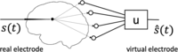
A real electrode (left) is selectively sensitive to brain sources near its tip and blind to distant sources. A virtual electrode (right) attempts to reproduce this property by applying a spatial filter u to the multichannel observation.
The aim of this paper is to facilitate this understanding, underscoring both the power of spatial filtering and its limits.
A Diversity of Filters
A variety of filters have been used to achieve different goals (Fig. 1C). A spatial filter might (1) enhance specific activity of interest or (2) suppress specific interference. Alternatively, it might merely (3) rearrange the data, for example, to reduce their dimensionality, orthogonalize the matrix of time series (remove correlations between channels), or even spatially “whiten” the data (i.e., transform it into a matrix with orthogonal columns of equal variance). Differential and CSD filters enhance local gradients, and they and rereferencing are useful to remove common-mode interference. PCA concentrates data variance in the first few components, and beamforming implements a virtual electrode as it is moved through source space (each column in the rightmost panel of Fig. 1B targets a different location).
Note that a spatial filter does not affect the spectral content of the data, other than by giving different weights to channels with different spectral contents. It does not remove, for instance, a so-called direct current (DC) bias, nor does it implement nonlinear transforms as it might arise within a neural network for the purpose of classification.
A virtual electrode (or “virtual sensor”) is a filter that aims to reproduce the spatial selectivity of a real electrode inserted into neural tissue (Fig. 2). Some empirical success has been reported, for example, in recovering the position and time course of sources picked up with real electrodes in epileptic patients undergoing presurgical recording with stereotactic EEG (sEEG) electrodes inserted deep in the brain (Juárez-Martinez et al., 2018; Alberto et al., 2021; Cao et al., 2022; Velmurugan et al., 2022; Coelli et al., 2023).
A simple argument tells us that a virtual electrode is not the same as a real electrode. If you placed a very large number
of real electrodes at different spots in the brain—say, one in each of the ∼120,000 cubic millimeters of the human brain—you
could in principle measure as many independent signals. If you tried to imitate those electrodes using “virtual electrodes”
based on a smaller number of real electrodes, you would run into a hard limit: you cannot create more independent information
than what the real electrodes provide, no matter how cleverly you combine their signals. In mathematical terms, whereas the
rank of data measured from real electrodes could be as large as their number <mml:math display="inline"><mml:msup><mml:mi>J</mml:mi><mml:mrow><mml:mi mathvariant="normal">′</mml:mi></mml:mrow></mml:msup></mml:math>J′
, the rank of data measured from the same number virtual electrodes cannot exceed
J, the number of actual electrodes or sensors. If <mml:math display="inline"><mml:mi>J</mml:mi><mml:mo><</mml:mo><mml:msup><mml:mi>J</mml:mi><mml:mrow><mml:mi mathvariant="normal">′</mml:mi></mml:mrow></mml:msup></mml:math>J<J′
, these data matrices are necessarily different, and thus virtual electrodes cannot be the same as real electrodes.
A similar argument can be made with respect to electromagnetic source imaging. At any point in time, only
J measured values are available to construct the <mml:math display="inline"><mml:msup><mml:mi>J</mml:mi><mml:mrow><mml:mi mathvariant="normal">′</mml:mi></mml:mrow></mml:msup><mml:mo>≫</mml:mo><mml:mi>J</mml:mi></mml:math>J′≫J
pixels or voxels of an “image” and, likewise, the time course of any pixel or voxel is a function of just
J sensor signals, in contrast to the <mml:math display="inline"><mml:msup><mml:mi>J</mml:mi><mml:mrow><mml:mi mathvariant="normal">′</mml:mi></mml:mrow></mml:msup></mml:math>J′
time courses—potentially independent—of the pixels or voxels of an optical imaging technique. These limitations are, of course,
well known: they reflect the fundamental nonuniqueness of the inverse problem (Baillet, 2010). As in other scientific fields—and indeed perception itself (Helmholtz, 1867)—additional assumptions are required in the form of an internal model constrained by the observations to allow inference of source activity or locations. This works well: witness the success of electromagnetic imaging methods in neuroscience
(Baillet, 2010).
Nevertheless, we may (indeed we should) feel uneasy using the outcome of an inference process as evidence, because the degree to which that evidence reflects the observed data, as opposed to the priors included in the inference model, is unclear (Tarantola, 2006). Is the sharp boundary of activity, apparent in the image, a reflection of the data, or of the prior? Relatedly, are the imperfections that we observe due to method-related or equipment-related limitations (amenable to progress) or fundamental constraints (not amenable to progress). A goal of this paper is to help answer such questions or, at least, formulate them.
Some Theory
The aim of this section is to point out some basic properties of spatial filters and gain an intuitive understanding of what they can and cannot do. The same ideas are illustrated visually in the next section; the busy reader might want to skip forward and come back for reference.
Recorded data take the form of a matrix
X of size <mml:math display="inline"><mml:mi>T</mml:mi><mml:mo>×</mml:mo><mml:mi>J</mml:mi></mml:math>T×J
where
T is the number of samples and
J the number of channels (electrodes or sensors). The recorded data are assumed to reflect the activity of
I sources within the brain via a linear mixing process:<mml:math display="block"><mml:mspace width="0.25em"></mml:mspace><mml:mspace width="0.25em"></mml:mspace><mml:msub><mml:mi>x</mml:mi><mml:mi>j</mml:mi></mml:msub><mml:mo
stretchy="false">(</mml:mo><mml:mi>t</mml:mi><mml:mo stretchy="false">)</mml:mo><mml:mo>=</mml:mo><mml:munder><mml:mrow><mml:mo
movablelimits="false">∑</mml:mo></mml:mrow><mml:mi>i</mml:mi></mml:munder><mml:mspace width="0.2em"></mml:mspace><mml:msub><mml:mi>m</mml:mi><mml:mrow><mml:mi>i</mml:mi><mml:mi>j</mml:mi></mml:mrow></mml:msub><mml:msub><mml:mi>s</mml:mi><mml:mi>i</mml:mi></mml:msub><mml:mo
stretchy="false">(</mml:mo><mml:mi>t</mml:mi><mml:mo stretchy="false">)</mml:mo><mml:mo>,</mml:mo><mml:mspace width="2em"></mml:mspace><mml:mo
stretchy="false">(</mml:mo><mml:mn>1</mml:mn><mml:mo stretchy="false">)</mml:mo></mml:math>xj(t)=∑imijsi(t),(1)
in matrix notation <mml:math display="inline"><mml:mrow><mml:mi mathvariant="bold">X</mml:mi></mml:mrow><mml:mo>=</mml:mo><mml:mrow><mml:mi mathvariant="bold">S</mml:mi><mml:mi
mathvariant="bold">M</mml:mi></mml:mrow></mml:math>X=SM
, where
S of size <mml:math display="inline"><mml:mi>T</mml:mi><mml:mo>×</mml:mo><mml:mi>I</mml:mi></mml:math>T×I
represents the activity of the sources and
M is a mixing matrix of size <mml:math display="inline"><mml:mi>I</mml:mi><mml:mo>×</mml:mo><mml:mi>J</mml:mi></mml:math>I×J
. It is common in the literature to see a noise term added to this equation (e.g., <mml:math display="inline"><mml:mrow><mml:mi mathvariant="bold">X</mml:mi></mml:mrow><mml:mo>=</mml:mo><mml:mrow><mml:mi mathvariant="bold">S</mml:mi><mml:mi
mathvariant="bold">M</mml:mi></mml:mrow><mml:mo>+</mml:mo><mml:mrow><mml:mi mathvariant="bold">N</mml:mi></mml:mrow></mml:math>X=SM+N
) but here noise sources are included in
S. The matrix
X is observed, whereas
S and
M can only be inferred.
We are usually interested in the activity of certain brain sources, i.e., one or more columns of
S. Since the sources were mixed linearly, it makes sense to try to recover them using linear demixing methods. Typically,
an analysis matrix
U of size <mml:math display="inline"><mml:mi>J</mml:mi><mml:mo>×</mml:mo><mml:mi>K</mml:mi></mml:math>J×K
is applied to the data to yield a matrix
Y of size <mml:math display="inline"><mml:mi>T</mml:mi><mml:mo>×</mml:mo><mml:mi>K</mml:mi></mml:math>T×K
of transformed data:<mml:math display="block"><mml:mspace width="0.25em"></mml:mspace><mml:msub><mml:mi>y</mml:mi><mml:mi>k</mml:mi></mml:msub><mml:mo
stretchy="false">(</mml:mo><mml:mi>t</mml:mi><mml:mo stretchy="false">)</mml:mo><mml:mo>=</mml:mo><mml:munder><mml:mrow><mml:mo
movablelimits="false">∑</mml:mo></mml:mrow><mml:mi>j</mml:mi></mml:munder><mml:mspace width="0.2em"></mml:mspace><mml:msub><mml:mi>u</mml:mi><mml:mrow><mml:mspace
width=".1em"></mml:mspace><mml:mi>j</mml:mi><mml:mi>k</mml:mi></mml:mrow></mml:msub><mml:msub><mml:mi>x</mml:mi><mml:mi>y</mml:mi></mml:msub><mml:mo
stretchy="false">(</mml:mo><mml:mi>t</mml:mi><mml:mo stretchy="false">)</mml:mo><mml:mo>,</mml:mo><mml:mspace width="2em"></mml:mspace><mml:mo
stretchy="false">(</mml:mo><mml:mn>2</mml:mn><mml:mo stretchy="false">)</mml:mo></mml:math>yk(t)=∑jujkxy(t),(2)
in matrix notation <mml:math display="inline"><mml:mrow><mml:mi mathvariant="bold">Y</mml:mi></mml:mrow><mml:mo>=</mml:mo><mml:mrow><mml:mi mathvariant="bold">X</mml:mi><mml:mi
mathvariant="bold">U</mml:mi></mml:mrow></mml:math>Y=XU
. Each column of
Y (a time series) is referred to here as a component.
K can be smaller or larger than
J; however if it is larger, the components are linearly dependent and thus correlated: the rank of
Y cannot be greater than that of
X.
Ideally, we would like the analysis matrix
U to be a “demixing matrix” so that <mml:math display="inline"><mml:mrow><mml:mi mathvariant="bold">M</mml:mi><mml:mi mathvariant="bold">U</mml:mi></mml:mrow><mml:mo>=</mml:mo><mml:mrow><mml:mi
mathvariant="bold">I</mml:mi></mml:mrow></mml:math>MU=I
, the identity matrix. Each column of
Y would then map to a source. Unfortunately, brain sources number in billions, whereas sensor channels range from tens to
thousands (i.e., <mml:math display="inline"><mml:mi>I</mml:mi><mml:mo>≫</mml:mo><mml:mi>J</mml:mi></mml:math>I≫J
), so
M is not invertible and therefore recovering
S is impossible. We must settle for the less ambitious objective of finding a transform that produces components that are
somehow more informative than the raw data. For example, a column of
Y might approximate the activity of a particular source, or the compound activity of several sources with a functional meaning
such as an event-related potential (ERP). Often, we are interested only in one such time series, and thus in just one column
u of the analysis matrix which constitutes a spatial filter, a vector of weights of size
J which, applied to the observations, produces a single, univariate time series.
Vector space
It is helpful to see neural activity, or recorded data, or filters, as belonging to a vector space. This allows for convenient short-cuts and useful insights thanks to concepts such as subspace, span, dimension, linear dependence, and orthogonality. For example, the brain source signals <mml:math display="inline"><mml:msub><mml:mi>s</mml:mi><mml:mi>i</mml:mi></mml:msub><mml:mo stretchy="false">(</mml:mo><mml:mi>t</mml:mi><mml:mo
stretchy="false">)</mml:mo></mml:math>si(t)
span a signal space that contains all of their linear combinations. Its dimension is at most
I, number of sources (it might be smaller if some of the <mml:math display="inline"><mml:msub><mml:mi>s</mml:mi><mml:mi>i</mml:mi></mml:msub><mml:mo stretchy="false">(</mml:mo><mml:mi>t</mml:mi><mml:mo
stretchy="false">)</mml:mo></mml:math>si(t)
are linearly dependent). The observed data <mml:math display="inline"><mml:msub><mml:mi>x</mml:mi><mml:mi>j</mml:mi></mml:msub><mml:mo stretchy="false">(</mml:mo><mml:mi>t</mml:mi><mml:mo
stretchy="false">)</mml:mo></mml:math>xj(t)
span a subspace of that space, of dimension at most
J, number of sensors. The mixing matrix
M projects from the source space onto this subspace. Since <mml:math display="inline"><mml:mi>I</mml:mi><mml:mo>≫</mml:mo><mml:mi>J</mml:mi><mml:mo>,</mml:mo></mml:math>I≫J,
a given observation <mml:math display="inline"><mml:msub><mml:mi>x</mml:mi><mml:mi>j</mml:mi></mml:msub><mml:mo stretchy="false">(</mml:mo><mml:mi>t</mml:mi><mml:mo
stretchy="false">)</mml:mo></mml:math>xj(t)
might reflect many different patterns of brain activity, a manifestation of the nonuniqueness mentioned earlier. This is
schematized in Figure 3, which shows how two different brain sources might give rise to the same observation when projected on to the lower-dimension
observation space.

The space spanned by the columns of the observation matrix X is a subspace of the space spanned by the brain signals S. Brain source signals are projected onto this subspace, and thus multiple sources may map onto the same observation, implying nonuniqueness of the inverse problem (Baillet, 2010).
Components (columns of
Y) also belong to the observation subspace spanned by the columns <mml:math display="inline"><mml:msub><mml:mi>x</mml:mi><mml:mi>j</mml:mi></mml:msub><mml:mo stretchy="false">(</mml:mo><mml:mi>t</mml:mi><mml:mo
stretchy="false">)</mml:mo></mml:math>xj(t)
of
X. For some analysis methods (e.g., PCA), the columns of
Y are mutually uncorrelated, in which case the subspace spanned by any subset of columns is orthogonal to the subspace spanned by the other columns. In other words, each vector (signal) in one subspace is uncorrelated with every vector in the other subspace:<mml:math display="block"><mml:munder><mml:mrow><mml:mo movablelimits="false">∑</mml:mo></mml:mrow><mml:mi>t</mml:mi></mml:munder><mml:mspace
width="0.2em"></mml:mspace><mml:msub><mml:mi>y</mml:mi><mml:mi>j</mml:mi></mml:msub><mml:mo stretchy="false">(</mml:mo><mml:mi>t</mml:mi><mml:mo
stretchy="false">)</mml:mo><mml:msub><mml:mi>y</mml:mi><mml:mrow><mml:mspace width=".1em"></mml:mspace><mml:msup><mml:mi>j</mml:mi><mml:mrow><mml:mi
mathvariant="normal">′</mml:mi></mml:mrow></mml:msup></mml:mrow></mml:msub><mml:mo stretchy="false">(</mml:mo><mml:mi>t</mml:mi><mml:mo
stretchy="false">)</mml:mo><mml:mspace width="0.25em"></mml:mspace><mml:mo>=</mml:mo><mml:mn>0.</mml:mn><mml:mspace width="2em"></mml:mspace><mml:mo
stretchy="false">(</mml:mo><mml:mn>3</mml:mn><mml:mo stretchy="false">)</mml:mo></mml:math>∑tyj(t)yj′(t)=0.(3)
Spatial filter, null filter, and zero set
As mentioned earlier, a spatial filter is a vector of
J weights <mml:math display="inline"><mml:mo stretchy="false">[</mml:mo><mml:mrow><mml:msub><mml:mi>u</mml:mi><mml:mi>j</mml:mi></mml:msub></mml:mrow><mml:mo
stretchy="false">]</mml:mo></mml:math>[uj]
to be applied to the observation channels. Since a linear combination of filters is a filter, spatial filters form a vector
space, and because there are
J coefficients, this space is of dimension
J.
Given a source
i, the source-to-filter-output gain for that source is as follows:<mml:math display="block"><mml:msub><mml:mi>g</mml:mi><mml:mi>i</mml:mi></mml:msub><mml:mo>=</mml:mo><mml:munder><mml:mrow><mml:mo
movablelimits="false">∑</mml:mo></mml:mrow><mml:mi>j</mml:mi></mml:munder><mml:mspace width="0.2em"></mml:mspace><mml:msub><mml:mi>m</mml:mi><mml:mrow><mml:mi>i</mml:mi><mml:mi>j</mml:mi></mml:mrow></mml:msub><mml:msub><mml:mi>u</mml:mi><mml:mi>j</mml:mi></mml:msub><mml:mo>.</mml:mo><mml:mspace
width="2em"></mml:mspace><mml:mo stretchy="false">(</mml:mo><mml:mn>4</mml:mn><mml:mo stretchy="false">)</mml:mo></mml:math>gi=∑jmijuj.(4)
This gain is a scalar, equal to the weighted sum of the gains from the source to each sensor. A null filter
u for a source is a filter for which the source-to-filter-output gain is zero:<mml:math display="block"><mml:munder><mml:mrow><mml:mo movablelimits="false">∑</mml:mo></mml:mrow><mml:mi>j</mml:mi></mml:munder><mml:mspace
width="0.2em"></mml:mspace><mml:msub><mml:mi>m</mml:mi><mml:mrow><mml:mi>i</mml:mi><mml:mi>j</mml:mi></mml:mrow></mml:msub><mml:msub><mml:mi>u</mml:mi><mml:mi>j</mml:mi></mml:msub><mml:mo>=</mml:mo><mml:mn>0</mml:mn><mml:mo>,</mml:mo><mml:mspace
width="2em"></mml:mspace><mml:mo stretchy="false">(</mml:mo><mml:mn>5</mml:mn><mml:mo stretchy="false">)</mml:mo></mml:math>∑jmijuj=0,(5)
i.e., the filter suppresses that source. For any source, a null filter for that source exists as long as there are at least
two sensors <mml:math display="inline"><mml:mo stretchy="false">(</mml:mo><mml:mi>J</mml:mi><mml:mo>></mml:mo><mml:mn>1</mml:mn><mml:mo
stretchy="false">)</mml:mo></mml:math>(J>1)
, a trivial example being a filter with all coefficients zero except for two channels
j and <mml:math display="inline"><mml:msup><mml:mrow><mml:mspace width=".1em"></mml:mspace><mml:mi>j</mml:mi></mml:mrow><mml:mrow><mml:mi
mathvariant="normal">′</mml:mi></mml:mrow></mml:msup></mml:math>j′
such that <mml:math display="inline"><mml:msub><mml:mi>u</mml:mi><mml:mi>j</mml:mi></mml:msub><mml:mo>/</mml:mo><mml:msub><mml:mi>u</mml:mi><mml:mrow><mml:msup><mml:mrow><mml:mspace
width=".1em"></mml:mspace><mml:mi>j</mml:mi></mml:mrow><mml:mrow><mml:mi mathvariant="normal">′</mml:mi></mml:mrow></mml:msup></mml:mrow></mml:msub><mml:mo>=</mml:mo><mml:mo>−</mml:mo><mml:mspace
width="0.25em"></mml:mspace><mml:msub><mml:mi>m</mml:mi><mml:mrow><mml:mi>i</mml:mi><mml:mi>j</mml:mi></mml:mrow></mml:msub><mml:mo>/</mml:mo><mml:mspace
width="0.25em"></mml:mspace><mml:msub><mml:mi>m</mml:mi><mml:mrow><mml:mi>i</mml:mi><mml:msup><mml:mi>j</mml:mi><mml:mrow><mml:mi
mathvariant="normal">′</mml:mi></mml:mrow></mml:msup></mml:mrow></mml:msub></mml:math>uj/uj′=−mij/mij′
. A weighted sum of null filters is obviously a null filter, and thus the null filters for any given source form a vector
space, subspace of the space of all spatial filters for
J channels. The dimension of that subspace is <mml:math display="inline"><mml:mi>J</mml:mi><mml:mo>−</mml:mo><mml:mn>1</mml:mn></mml:math>J−1
(the constraint of Eq. 5 reduces the dimension by one): in practical terms, a source typically has many null filters. Spatial filters are good at producing a signal that is “blind” to a source.
Given a second source <mml:math display="inline"><mml:msup><mml:mi>i</mml:mi><mml:mrow><mml:mi mathvariant="normal">′</mml:mi></mml:mrow></mml:msup></mml:math>i′
, there exists likewise a subspace of null filters of dimension <mml:math display="inline"><mml:mi>J</mml:mi><mml:mo>−</mml:mo><mml:mn>1</mml:mn></mml:math>J−1
for that second source. The null filters for both sources belong to the intersection of their subspaces, i.e., to a subspace
of dimension <mml:math display="inline"><mml:mi>J</mml:mi><mml:mo>−</mml:mo><mml:mn>2</mml:mn></mml:math>J−2
. Repeating this argument, for
J observation channels one can suppress up to <mml:math display="inline"><mml:mi>J</mml:mi><mml:mo>−</mml:mo><mml:mn>1</mml:mn></mml:math>J−1
arbitrarily-positioned sources. The filter that does so belong to a subspace of dimension one, i.e., that filter is unique to a multiplicative factor. For a greater number of sources, we cannot guarantee the existence of a filter that suppresses
them all. In general, at most <mml:math display="inline"><mml:mi>J</mml:mi><mml:mo>−</mml:mo><mml:mn>1</mml:mn></mml:math>J−1
sources can be suppressed by a spatial filter applied to
J channels.
The zero set of a filter is the set of source locations for which the gain (Eq. 4) is zero. If the filter is a null filter for a particular source, its zero set obviously includes that source but, based on the reasoning that led to Figure 3, we expect other sources to have the same gain of zero. In other words, we expect the zero set to be extended in source space, as will be apparent in several of the figures below.
Data-driven analysis
Spatial filters can be hard-wired as mentioned earlier, but it is not always easy to guess coefficients that will work best
for a given set of data. Data-driven methods such as PCA, ICA, beamforming, or others offer a convenient way to find effective
coefficients. Among them, PCA stands out for three useful properties. First, the columns of the component matrix <mml:math display="inline"><mml:mrow><mml:mi mathvariant="bold">Y</mml:mi></mml:mrow><mml:mo>=</mml:mo><mml:mrow><mml:mi mathvariant="bold">X</mml:mi><mml:mi
mathvariant="bold">U</mml:mi></mml:mrow></mml:math>Y=XU
are mutually uncorrelated (Eq. 3). Second, their variance adds up to the variance of
X. Third, the first principal component packs the largest possible amount of variance, the second the largest amount of variance
in the subspace orthogonal to the first, and so on. A consequence of this third property is that the last principal component includes the least possible amount of variance and, indeed, if the data are rank-deficient, its variance is zero. Thus, if at most <mml:math display="inline"><mml:mi>J</mml:mi><mml:mo>−</mml:mo><mml:mn>1</mml:mn></mml:math>J−1
sources are active, the last column of the PCA matrix is a null filter for them all.
Other methods offer different properties (Parra et al., 2005). ICA attempts to ensure that components are statistically independent according to some empirical measure (Cardoso, 2001). Canonical correlation analysis (CCA) seeks linear combinations of columns of
X that are maximally correlated with some other dataset <mml:math display="inline"><mml:mrow><mml:msup><mml:mrow><mml:mi mathvariant="bold">X</mml:mi></mml:mrow><mml:mrow><mml:mi
mathvariant="normal">′</mml:mi></mml:mrow></mml:msup></mml:mrow></mml:math>X′
. Joint decorrelation (JD, also known as denoising source separation, DSS, or common spatial patterns, CSP) seeks to maximize
the ratio of variance between the data and a filtered version of the data (see de Cheveigné and Parra, 2014 and references therein). Beamforming applied to a source location produces a filter that minimizes variance at the output of the filter, subject that the gain
from the selected location (Eq. 4) is one. Data-driven analysis is discussed further in a later section.
Illustrations
A flat world
The previous concepts are somewhat abstract and it may be hard to see how they relate to actual measurements of neural data. In particular, it may be hard to grasp the relations between a signal space, the physical space that the sources and sensors inhabit, and the parameter space of a source model. Brain sources are often assimilated to dipoles located within a 5D parameter space (position and orientation) constrained to a convoluted shape (cortex), which is hard to visualize. The “flat world” presented here captures the essence of the problem and is easier to visualize.
The flat world consists of a disk-shaped source space with sensors at the periphery (Fig. 4A), a geometry simpler than that of a brain surrounded by MEG sensors or EEG electrodes (panel B). Source-to-sensor gain varies
with distance as <mml:math display="inline"><mml:mn>1</mml:mn><mml:mo>/</mml:mo><mml:msup><mml:mi>d</mml:mi><mml:mn>2</mml:mn></mml:msup></mml:math>1/d2
and there is no dependency on orientation, in contrast to EEG or MEG. Panel C shows the gain pattern of a single sensor,
and panel D shows the source-to-filter-output gain for a simple spatial filter with two nonzero coefficients, chosen to have
zero gain for a source at the cross. This filter is a null filter for that source, and the zero set of this filter includes the location of the source (cross) as well as other locations along a curved line (white). In contrast
to the simple patterns of panels C and D, the gain patterns of a single MEG sensor (panel E) and a two-sensor spatial filter
(panel F) are both convoluted, with bands of positive and negative gain according to relative orientations of sources and
sensors. If source orientations were free (as opposed to normal to the cortical surface, as here), the 5D parameter space
would be even harder to illustrate visually. The easier-to-visualize flat world captures the essence of the more complex system.

A, The “flat world” consists of a disk-shaped source space with sensors at the periphery. The source-to-sensor gain varies
with distance as <mml:math display="inline"><mml:mn>1</mml:mn><mml:mo>/</mml:mo><mml:msup><mml:mi>d</mml:mi><mml:mn>2</mml:mn></mml:msup></mml:math>1/d2
as represented by a color code at each sensor for a source located at the cross. B, The geometry of sources within the brain, and of sensors in a real MEG system are harder to visualize. The gain for each
MEG sensor relative to a source is coded as color (the dipolar source is positioned at the cross, oriented normally with respect
to the cortical surface, pointing inward). C, Gain pattern for a single sensor (red dot) as a function of source position in the flat world. D, Gain pattern for a simple spatial filter with two nonzero coefficients, chosen to ensure zero gain at the position of the
cross. E, Gain pattern for single MEG sensor (oblique red square) relative to dipolar sources as a function of their location on the
cortical surface. Sources are constrained to be normal to that surface. F, Gain pattern for a simple spatial filter with two nonzero coefficients with opposing sign (red and blue squares). All panels:
positive and negative gains are plotted on separate logarithmic scales, with small and large absolute values clipped for visual
clarity.
Null filters
Figure 5A shows the gain maps of four null filters for the source located at the cross. Their zero sets (white) have diverse shapes which all include the source location. These four null filters form a basis of the four-dimensional space of null filters for this source, i.e., any null filter is a weighted sum of these (one example being the filter of Fig. 3D).

A, Gain maps for four null filters for the source located at the cross. B, Three null filters for two sources. C, Two null filters for three sources. D, Unique null filter for four sources.
A word about how these particular filters were found: a Gaussian-distributed “source activity” matrix of size 1,000 × 1 was multiplied by the 1 × 5 source-to sensor gain matrix for the location indicated by the cross, resulting in a “data matrix” of size 1,000 × 5. PCA was applied, producing a 5 × 5 transform matrix. The last four columns of this matrix are null filters (Fig. 5A) for the source because the data matrix is of rank one. This illustrates the aforementioned process of deriving spatial filters by a data-driven method. For the 274-sensor MEG system of Figure 3B, there is likewise a 273-filter basis for the subspace of null filters for a source, but the gain pattern of any of these filters would be very hard to visualize.
Null filters for multiple sources
Figure 5B shows the gain maps of three null filters for two sources (crosses). Here, null filters form a subspace of dimension <mml:math display="inline"><mml:mi>J</mml:mi><mml:mo>−</mml:mo><mml:mn>2</mml:mn><mml:mo>=</mml:mo><mml:mn>3</mml:mn></mml:math>J−2=3
. Likewise, panels C and D show gain maps of null filters for three and four sources, respectively. The null filter for four
sources (panel D) is unique to a multiplicative constant. That filter can suppress additional sources if they fall within its zero set (white lines in
panel D), otherwise, in general, at most <mml:math display="inline"><mml:mi>J</mml:mi><mml:mo>−</mml:mo><mml:mn>1</mml:mn><mml:mo>=</mml:mo><mml:mn>4</mml:mn><mml:mspace
width="0.25em"></mml:mspace></mml:math>J−1=4
sources can be suppressed. For the 274-channel MEG system of Figure 3B, at most 273 arbitrarily located sources can be suppressed, and the filter that achieves this (without mapping everything
to zero) is also unique to a multiplicative factor.
A Virtual Electrode?
A real electrode has two properties that make it useful in scientific and clinical applications. First, the signal-to-noise ratio of the activity of a neural source (e.g., single neuron or epileptic focus) can be enhanced by placing the tip near that source. Second, a source can be located by “listening” for some expected activity while moving the tip around. For example, a primary sensory region might be located by advancing an electrode until stimulus-evoked spikes are heard over the loudspeaker. Ideally, we would like a virtual electrode to approximate both properties. Let us now look at each in turn.
Enhancement of signal-to-noise ratio (SNR)
The SNR is the ratio between the variance of the target (source of interest) and that of the background (all other sources).
In a simulation where target and background are known, the SNR can be calculated exactly at each sensor and at the output
of a spatial filter. We can then calculate the SNR enhancement ratio as the ratio between SNR at the filter output and the maximum SNR over sensors: a value greater than one indicates that the
filter offers a benefit over just selecting the best sensor. If the number of background sources is <mml:math display="inline"><mml:mi>J</mml:mi><mml:mo>−</mml:mo><mml:mn>1</mml:mn></mml:math>J−1
or less, a filter can be found that suppresses them all (as illustrated in Figs. 5 and 6A). If the target source is not located within the zero set of that filter, the enhancement ratio is infinite (if it is located within the zero set, the ratio is undefined because both target and background are suppressed). In the
more general case of
J or more background sources (as in real EEG or MEG recordings), the SNR enhancement ratio of the best possible filter will
depend on the geometry of all sensors and sources.
To illustrate the range of SNR enhancement ratios to expect, Figure 6 shows gain maps for filters designed to optimize the SNR of a target (circle) in the presence of interferers (crosses), for various configurations. To find these filters, a 10,000-row matrix of Gaussian noise was synthesized with as many columns as interferers, a target waveform was synthesized as a sinusoid with period 1,000 samples, the flat-world “forward model” was applied to these sources to create a data matrix with as many columns as sensors, and the JD algorithm was applied to those data to find the spatial filter that maximizes the variance ratio between trial-averaged data (each period counting as a trial) and the raw data.

Quantifying SNR enhancement in a flat world model. A–E, Gain patterns for spatial filters that optimize the SNR of a target (circle) in the presence of background sources (crosses) for various layouts of target, background and sensors. The SNR enhancement ratio is indicated for each plot.
The filter in panel A achieves infinite enhancement because, with 15 sensors, a spatial filter exists that perfectly suppresses the 14 interferers, and the target luckily does not fall within its zero set. For panels B-E, the SNR ratio depends on the configuration in a complex fashion: compare C and D with same sensor and target layout but different interferer positions, and B and E with the same target and interferer layout but different sensor positions. The bottom line is that (1) spatial filtering is always beneficial in terms of SNR and (2) the benefit depends strongly on the configuration.
Figure 7 shows analogous results for a simulation with real MEG data and an anatomy-informed source/forward model based on publicly available data from the BrainStorm tutorial (Tadel et al., 2011). That dataset included 274-channel MEG recordings in response to repeated tones in an auditory oddball task, together with co-registered anatomical and sensor information. A gain matrix was calculated based on an overlapping sphere model, each column representing the gain from one source location to each of the sensors. The model sources were dipoles that could be located in any of 135,002 positions on the cortical surface, with an orientation normal to the surface. For each dipole location in the model, a “target” source waveform was synthesized as a 1 Hz sinusoid with amplitude 30 nAm and multiplied by the corresponding column of the gain matrix, and the 274-channel result was added to the real MEG data. The real MEG data were used only as a realistic background for this simulation.

Quantifying SNR enhancement in a real 274-channel MEG configuration. A, SNR at the best sensor as a function of source location (left hemisphere viewed from the right, no transparency). B, SNR at the optimal filter output (same view). C, SNR enhancement ratio (same view). D, SNR enhancement as a function of depth (distance between a source and the closest sensor) for each source location. The red line indicates a quadratic fit to the log values.
For each source location, a LCMV beamformer solution was calculated to obtain an optimal filter to suppress the background while preserving the target. Figure 7A plots the maximum SNR over sensors (i.e., the best SNR achievable without spatial filtering) for each target location within the left hemisphere (viewed from the right, with the right hemisphere removed). As expected, the SNR tends to be better for superficial sources (red/yellow) than deep (blue). Panel B plots the SNR after spatial filtering: the SNR is improved for all target source locations, as confirmed by a plot of the SNR enhancement ratio (panel C). The enhancement ratio ranges across locations from ∼2 to ∼35 (median ∼5). Such values are of practical significance: an enhancement ratio of 5 is equivalent to multiplying by 25 the number of repeats in an evoked response paradigm.
This is both good news, and bad. The good news is that there is a benefit for every location. The bad news is that the size of the benefit is smaller than expected from a real electrode, if we could insert one into the brain. Also, it varies from one location to the next in a rather unpredictable fashion, reminiscent of the diversity observed in Figure 6. On average, the SNR improvement ratio is somewhat larger for superficial and deep sources than intermediate (Fig. 7D), but at every depth the spread of ratios is wide. The diversity likely reflects the fact that the zero set of the filter that attenuates the background has a complex geometry (as illustrated for the flat world in Fig. 6), and avoiding it is harder for some locations than others. Of course, the patterns of Figure 7 are specific to the dataset chosen: other datasets might yield different patterns, depending on sensor configurations, subjects, or recordings.
The analysis illustrated in Figure 7 requires anatomical information (e.g., MRI scan), together with a recording representative of the expected background activity, but it does not require recording the target activity itself. It might be useful to perform on a routine basis, so as to predict the benefit of a virtual electrode placed within a particular brain structure.
Source localization
A second useful property of a real electrode is the ability to locate a source by moving the electrode around until a particular response is observed. This property can be emulated by scanning a beamformer across the source space while monitoring its output. The location that yields the best SNR (according to some empirical measure) yields the position of the target source, as illustrated in Figure 8A. The SNR is indeed maximal at the correct position (circle), but the pattern does not taper off with distance as fast as for a real electrode, and the peak is rather broad. Regardless, the principle works: a source can be located by scanning a model source space with a beamformer, as long as there exists some criterion to detect when the filter output matches the target. Beamforming is one of several popular approaches to source localization (Baillet et al., 2001; Baillet, 2010; Jaiswal et al., 2020).

Locating a source by scanning with a beamformer. A, SNR as a function of the beamformer location parameter within the flat-world source space, for a target source (circle) in the presence of four competing sources (crosses). B, Gain map of the spatial filter found by the beamformer at the target location. C, SNR as a function of beamformer location parameter for a source located on the left-most node of a dipolar 274-channel MEG source model. D, Gain map of the beamformer solution when its location parameter coincides with the target source. SNR plots are in gray because values are uniformly positive; gain plots are in color because values can be positive or negative (in contrast to Fig. 7 which used color for both for visual clarity).
It is interesting to observe that the filter found at the target location (panel B) has the same gain pattern as that of Figure 5D, to a factor. Indeed, for <mml:math display="inline"><mml:mi>J</mml:mi><mml:mo>−</mml:mo><mml:mn>1</mml:mn></mml:math>J−1
competing sources (as here), the filter found by the beamformer will be the same for every target source position (other
than positions within the zero set of this filter). Thus, the gain pattern of this “virtual electrode” does not change as
it is moved around, counterintuitively and contrary to a real electrode. In the more realistic case of
J or more competing sources, the gain pattern will change with target position; however, we should not expect it to ever resemble the focal pattern of a real electrode.
Figure 8C shows the SNR of a spatial filter created by a beamformer as it is scanned across the parameter space of an MEG cortical source model. The data were created by placing a target source at the left-most location in the source model (roughly centered on the white zone in panel C), applying the forward model for that position, and adding the result to a background of real MEG data. Analogous to panel A (flat world), the SNR is maximal at the correct position, but again the pattern does not taper off as fast as for a real electrode. The gain pattern of the filter obtained by the beamformer pointed at the target is shown in panel D. Again, it does not resemble the focal gain pattern of a real electrode. The maximum gain is ∼10, implying that even for a beamformer focused on the target source, variance from the background (noise) sources leaks in to the filtered channel. If the source model used by the beamformer were inaccurate, the SNR gain would presumably be even smaller.
A Virtual Scalpel?
We are now aware that the ideal of a virtual electrode is incompletely attained. An alternative metaphor worth exploring,
however, is that of a “virtual scalpel” by which the activity of a source is silenced within the data. This, we saw, can be
achieved perfectly by a spatial filter (indeed there are many such filters, as they form a subspace of dimension <mml:math display="inline"><mml:mi>J</mml:mi><mml:mo>−</mml:mo><mml:mn>1</mml:mn></mml:math>J−1
of the space of filters). This suggests an alternative approach to analysis based on cancellation of individual sources.
This can take several forms.
A first is denoising, by which an unwanted source is projected out of the data, for example, by a denoising matrix defined as follows:<mml:math display="block"><mml:mrow><mml:mi mathvariant="bold">D</mml:mi></mml:mrow><mml:mo>=</mml:mo><mml:mrow><mml:mi mathvariant="bold">U</mml:mi><mml:mi
mathvariant="bold">E</mml:mi></mml:mrow><mml:msup><mml:mrow><mml:mi mathvariant="bold">U</mml:mi></mml:mrow><mml:mrow><mml:mo>−</mml:mo><mml:mn>1</mml:mn></mml:mrow></mml:msup><mml:mo>,</mml:mo><mml:mspace
width="2em"></mml:mspace><mml:mo stretchy="false">(</mml:mo><mml:mn>6</mml:mn><mml:mo stretchy="false">)</mml:mo></mml:math>D=UEU−1,(6)
where <mml:math display="inline"><mml:msup><mml:mrow><mml:mi mathvariant="bold">U</mml:mi></mml:mrow><mml:mrow><mml:mo>−</mml:mo><mml:mn>1</mml:mn></mml:mrow></mml:msup></mml:math>U−1
is the inverse (or pseudoinverse) of the transform matrix
U and
E is a diagonal matrix with ones for components to retain and zeros for components to remove. Applying this to the data yields
a “clean” data matrix <mml:math display="inline"><mml:mrow><mml:mover><mml:mrow><mml:mi mathvariant="bold">X</mml:mi></mml:mrow><mml:mo stretchy="false">^</mml:mo></mml:mover></mml:mrow><mml:mo>=</mml:mo><mml:mrow><mml:mi
mathvariant="bold">X</mml:mi><mml:mi mathvariant="bold">D</mml:mi></mml:mrow></mml:math>X^=XD
. This matrix has the same size as the original data and can be substituted for it in further analyses, with two caveats.
First <mml:math display="inline"><mml:mrow><mml:mover><mml:mrow><mml:mi mathvariant="bold">X</mml:mi></mml:mrow><mml:mo stretchy="false">^</mml:mo></mml:mover></mml:mrow></mml:math>X^
is not of full rank. Second, if further analyses call for a forward model, that model may need to be adjusted for effects
of the denoising matrix (Hipp and Siegel, 2015). An example of this approach is the common use of ICA to isolate and remove ocular artifacts; another is that of JD to remove
eyeblinks or power line artifacts.
A second approach is illustrated in Figure 9 for a flat-world simulation of a stimulus-evoked response involving two sources. In real brain data, it is common to find multiple spatiotemporal components because sources in different hemispheres or in lower- versus higher-order cortical fields may have different latencies or time constants. Their time courses are often correlated, and it may be hard to separate one from the other. Here, the simulation includes two target sources (circles in lower parts of panels C–E) driven with distinct but correlated waveforms (panel A) that repeat periodically and three competing sources (crosses in lower parts of panels C–E) driven with independent Gaussian noise.

A, Time courses of target sources (with locations indicate as circles in panels C, D. B, Mixture. C, Time courses of components retrieved by JD (top) and maps of filters associated with those components (bottom). D, Time courses of components rotated by a second application of JD to isolate the later source (top) and corresponding filter (bottom). E, Time courses of components rotated by a third application of JD to isolate the earlier source (top) and corresponding filter (bottom). The latter two filters (#3 and #4) have the property that they cancel all sources but one, which they thus isolate, a property that filters produced by the initial JD (#1 and #2) lack.
The sources were mixed with source-to-sensor gains appropriate for their positions, resulting in the mixture shown in panel B. A first JD analysis was applied to separate the targets from the noise, resulting in two components (panel C), both clean of noise but neither of which matches a source (the corresponding filters have nonzero gain at both source locations).
A second JD analysis was then applied to these two components to find an “early component” active from 1–100 samples. The first component of this analysis (panel D, blue) is again a mixture, but the second component (red) matches source 2 (indeed, the filter shown in the lower part of the panel cancels all but that source). A third JD analysis applied to find a “late” component (active from 201–400 samples) likewise found a component matching source 1. Combining these analyses, both sources can be isolated. This approach is in principle applicable to real EEG or MEG data, but the outcome is harder to validate for lack of ground truth.
A third approach exploits the fact that a source is necessarily located at the intersection of the zero sets of all its null filters to localize it (de Cheveigné, 2024). These examples show how spatial filters might be used as sort of “virtual scalpel” to dissect complex brain activity. The first (denoising) is well established; the others are less thoroughly validated at this point.
Finding a Filter
Preceding sections focused on the properties of spatial filters; this section revisits how they are found. Note that this is a hard problem: trying just two values for each of 274 coefficients would require roughly as many trials as there are atoms in the universe, ∼1082.
Predetermined (hard-wired)
Filter weights are chosen based on prior knowledge. For example, common-mode interference that affects all channels might be attenuated by subtracting one particular channel or a combination of channels (rereferencing). If the interference is known to vary slowly across space (as for a distant environmental source in MEG), a differential montage may be useful (e.g., gradiometers in MEG). The spatial model can be more sophisticated, as in the SSS method (Taulu and Simola, 2006), implemented under the name of MaxFilter in certain MEG systems. In that method, the magnetic field is decomposed on a basis of spherical harmonics centered on the subject's head, and this decomposition is used to determine weights to apply to the sensors that sample the field. The basis is partitioned into components likely to arise from within the head, which are retained, and those likely to arise from outside, which are discarded.
Data-driven
PCA involves eigen-decomposition of the empirical covariance matrix of the data (Greenacre et al., 2022), while JD involves joint eigen-decomposition of two covariance matrices (de Cheveigné and Parra, 2014 and references therein). Likewise, CCA exploits the covariance matrix of two concatenated datasets (de Cheveigné et al., 2018 and references therein). Each of these methods “sees” the data through statistics that capture the correlation structure of the data (which itself reflects mixing of the same brain sources into multiple channels, Eq. 1). In addition to covariance, ICA may exploit higher-order statistics. None of these methods uses sensor location or anatomical information, and there is no assumption on the number or nature of the sources.
Hybrid (beamformer)
The LCMV beamformer solution for source location
i is obtained as follows:<mml:math display="block"><mml:mrow><mml:mi mathvariant="bold">u</mml:mi></mml:mrow><mml:mo>=</mml:mo><mml:mo stretchy="false">(</mml:mo><mml:msubsup><mml:mrow><mml:mi
mathvariant="bold">f</mml:mi></mml:mrow><mml:mi>i</mml:mi><mml:mo>⊺</mml:mo></mml:msubsup><mml:msup><mml:mrow><mml:mi mathvariant="bold">C</mml:mi></mml:mrow><mml:mrow><mml:mo>−</mml:mo><mml:mn>1</mml:mn></mml:mrow></mml:msup><mml:msub><mml:mrow><mml:mi
mathvariant="bold">f</mml:mi></mml:mrow><mml:mi>i</mml:mi></mml:msub><mml:msup><mml:mo stretchy="false">)</mml:mo><mml:mrow><mml:mo>−</mml:mo><mml:mn>1</mml:mn></mml:mrow></mml:msup><mml:msub><mml:mrow><mml:mi
mathvariant="bold">f</mml:mi></mml:mrow><mml:mi>i</mml:mi></mml:msub><mml:msup><mml:mrow><mml:mi mathvariant="bold">C</mml:mi></mml:mrow><mml:mrow><mml:mo>−</mml:mo><mml:mn>1</mml:mn></mml:mrow></mml:msup><mml:mo>,</mml:mo><mml:mspace
width="2em"></mml:mspace><mml:mo stretchy="false">(</mml:mo><mml:mn>7</mml:mn><mml:mo stretchy="false">)</mml:mo></mml:math>u=(fi⊺C−1fi)−1fiC−1,(7)
where
u is the spatial filter, <mml:math display="inline"><mml:msub><mml:mrow><mml:mi mathvariant="bold">f</mml:mi></mml:mrow><mml:mi>i</mml:mi></mml:msub></mml:math>fi
is the source-to-sensor gain for that location, and
C is, again, the covariance matrix of observed multichannel data (Van Veen et al., 1997; Jaiswal et al., 2020). Here, statistics from the data are complemented by a source/forward model which captures known geometry and anatomical
constraints. The added constraint from anatomical information can be a plus (unrealistic solutions are avoided) or a minus
(an optimal filter might not be found if the target does not fit the source model).
Potential Problems
Existence versus identifiability
Data-driven analysis can fail for two reasons: (1) the desired solution does not exist, due to a fundamental constraint, or (2) the desired solution exists but we fail to find it, for example, due to geometrical inaccuracy, or lack of appropriate criteria, or overfitting. In the second case, a new technique might overcome the limitation; in the first, it cannot. It is useful to distinguish these two situations.
Overfitting
Overfitting occurs when there are insufficient data to properly constrain the parameters. An oft-quoted rule of thumb is that
at least <mml:math display="inline"><mml:mn>10</mml:mn><mml:mi>J</mml:mi></mml:math>10J
time points are needed for
J parameters, but the theoretical basis for that rule is weak (Siegel, 2022). In particular, overfitting may be less severe if inter-channel correlation allows the number of free parameters to be reduced, or more severe if the data have serial correlation, as this implies fewer “effective samples.” Indeed, brain data often have roughly <mml:math display="inline"><mml:mn>1</mml:mn><mml:mo>/</mml:mo><mml:mi>f</mml:mi></mml:math>1/f
spectra and thus strong serial correlation. Overfitting entails both a risk of unsound observations (the analysis latches
on to a quirk) and a loss of sensitivity in the cross-validation stage (the analysis fails to recognize a real effect). I
recommend a three-pronged approach:
-
Proactively look for factors that promote overfitting, and evidence that it might be occurring. Are the results too good to be true?
-
Deploy standard cross-validation techniques (Varoquaux et al., 2017), such as training on a subset of the data and testing on another. Cross-validated results are less likely to be spurious.
-
Reduce dimensionality and/or apply regularization.
Cross-validation by itself does not “cure” overfitting. Rather, it reduces the risk of reporting a false result but also makes analysis less sensitive to a real effect. Dimensionality reduction reduces the overfitting itself, although it also entails the risk of removing relevant information.
Is data-driven analysis safe?
Empirical sciences ask questions of the data, the foremost of which is whether an observed pattern is real, that is, it reflects an interesting phenomenon rather than a random quirk. A tool such as spatial filtering may help by reducing randomness and increasing the SNR of real patterns; however, we must be worried when that tool itself depends on the data. For example, the JD algorithm is useful to find a spatial filter that isolates stimulus-evoked response components from multichannel neural data (de Cheveigné and Parra, 2014). Applied to random data, it will oblige by discovering chance directions that happen to be similar over trials. The investigator must be alert (if not paranoid) to such “double-dipping” (Kriegeskorte et al., 2009; Gross et al., 2013; Devezer et al., 2021). Data-driven analysis is not safe: it requires attention.
What else can go wrong?
Disconcertingly, noise from one channel can be injected by a spatial filter into other channels. This is easily understood in the case of rereferencing: an artifact on the new reference (e.g., myogenic) will invade channels that were previously clean, with patterns that seem all the more “real” as they are now seen on multiple channels. However, the phenomenon can arise with any form of spatial filtering, often unexpectedly due to the hands-off nature of data-driven methods. There is no easy fix, other than be attentive to the phenomenon, and weigh the benefit of removing one source of noise against introducing another.
Tips and Tricks
In what order?
Spatial filtering is typically one step among several in a pipeline. Linear steps such as spatial or temporal filtering can be swapped, but nonlinear steps (as involved to find a data-driven solution) cannot. For example, PCA followed by temporal filtering will not yield the same outcome as if temporal filtering comes first. Spatial filtering entails reducing the variance of background sources, but if some of that variance is first removed by other means (e.g., high-pass filtering), parameters are freed to obtain a better spatial filter to remove the rest. Likewise, if high-amplitude glitches are removed first, the algorithm will not waste parameters trying to attenuate them but, on the other hand, applying spatial filtering first might make those glitches easier to identify and remove. The order of operations counts, but there is no universal rule: in each situation a careful consideration of processing order may yield better results.
Stepwise dimensionality reduction
Dimensionality reduction reduces overfitting and speeds computation; however, there is the risk of discarding informative dimensions by mistake. Furthermore, a data-driven dimensionality reduction operation may itself be prone to overfitting. An approach that I like to use is to operate in steps, each relatively conservative. For example, PCA can be applied to remove dimensions with variance below the floor of instrumental noise. This step is relatively safe. It can be preceded by SCA (shared component analysis, de Cheveigné, 2021) to down-weight variance specific to single channels (unlikely to reflect a neural source) and/or followed by JD to remove spatial components dominated by variance in an irrelevant spectral region, etc. For this approach to be of benefit, it is critical to verify that the criteria used to prioritize dimensions are distinct from effects tested in the study, to avoid “double-dipping.”
Boosting performance
A data-driven filter is the result of a compromise among various sources of variance to remove. The terms of this compromise can be improved in several ways. One is to first reduce the background variance by other means, as mentioned above. As an example, repeating the simulation of Figure 7 with a 30 Hz low-pass filter applied to the MEG background would increase the median SNR enhancement ratio by a factor of two, which, added to direct effects of low-pass filtering, would boost SNR by a factor close to three. If activity above 30 Hz were not of interest, such initial low-pass filtering would be a good move.
A second route to better performance is to start with data of greater dimensionality J. Adding more sensors increases the number of sources that can be suppressed, with two caveats (in addition to cost): each sensor contributes its own noise, adding to the count of sources to be cancelled, and it also increases risks of overfitting. If these factors are controlled for, increasing the number of sensors or electrodes is beneficial.
Data dimensionality can be increased in other ways. Taking advantage of the temporal sparsity of many sources, a different filter may be applied to different partitions of the time axis. With
N intervals, the effective dimensionality jumps to <mml:math display="inline"><mml:mi>N</mml:mi><mml:mi>J</mml:mi></mml:math>NJ
. Alternatively, the data may be filtered into different frequency regions, each with a different spatial filter. This approach
can be generalized by augmenting the data with time shifts <mml:math display="inline"><mml:mo stretchy="false">[</mml:mo><mml:mn>0</mml:mn><mml:mo>⋯</mml:mo><mml:mi>N</mml:mi><mml:mo>−</mml:mo><mml:mn>1</mml:mn><mml:mo
stretchy="false">]</mml:mo></mml:math>[0⋯N−1]
(or some other convolutional basis): the J-coefficient spatial filter is then replaced by a NJ-coefficient spatiotemporal filter (multichannel finite-impulse-response filter). Yet another approach is to operate within a space of quadratic forms
based on cross-products of the form <mml:math display="inline"><mml:msub><mml:mi>x</mml:mi><mml:mi>j</mml:mi></mml:msub><mml:mo stretchy="false">(</mml:mo><mml:mi>t</mml:mi><mml:mo
stretchy="false">)</mml:mo><mml:msub><mml:mi>x</mml:mi><mml:mrow><mml:mspace width=".1em"></mml:mspace><mml:msup><mml:mi>j</mml:mi><mml:mrow><mml:mi
mathvariant="normal">′</mml:mi></mml:mrow></mml:msup></mml:mrow></mml:msub><mml:mo stretchy="false">(</mml:mo><mml:mi>t</mml:mi><mml:mo
stretchy="false">)</mml:mo></mml:math>xj(t)xj′(t)
. These can then be filtered by a J(J−1)/2-coefficient quadratic component analysis filter (QCA, de Cheveigné, 2012).
Each of these schemes entails increased risks of overfitting, the burden of mastering a more complex technique and explaining it to the reader, and time wasted “tinkering” with its various possibilities. It also increases researcher degrees of freedom, which should not be a deterrent but requires care when evaluating statistical significance (Kriegeskorte et al., 2009; Simmons et al., 2021).
Conclusion
Spatial filtering is an important tool for brain data analysis. It helps us in reversing the source-to-sensor mixing process that produced the data. As such, it is limited by the sparsity of observations that implies a nonuniqueness of the inverse problem (Baillet et al., 2001; Baillet, 2010). A well-chosen spatial filter can increase the SNR of sources of interest beyond that available at any of the sensors, which motivates the term “virtual electrode” to describe such a filter. However, it may be tempting to over-state this metaphor: noninvasive exploration is no stand-in for invasive exploration with a real electrode. What a spatial filter can do perfectly, however, is cancel a source (i.e., a “virtual scalpel”). A goal of this paper was to ease understanding of the algebraic, geometrical, physical, and computational constraints behind these ideas, which are often left obscured by the complex geometry of brain sources and sensors, and the high dimensionality of brain data.
Code availability
Matlab code for the “flat world” simulations is available at https://github.com/adc2/FlatWorld.
Footnotes
- Received April 24, 2025.
- Revision received January 5, 2026.
- Accepted January 10, 2026.
-
Malcolm Slaney, Lucas Parra, and Israel Nelken and two anonymous reviewers gave useful comments on earlier drafts. This work was supported by Agence Nationale de la Recherche grant ANR-17-EURE-0017.
-
The author declares no competing financial interest.
- Correspondence should be addressed to Alain de Cheveigné at alain.de.cheveigne{at}ens.fr.
- Copyright © 2026 the authors