Session 1 (localizer)

Pretraining 1. In the Session 1 pretraining, participants learned that each animal was associated with a specific food pellet. Food pellets were bidimensional stimuli composed of a shape and a texture. On each trial, participants were shown a short animal video (0.75 s), followed by a 0.5 s blank delay. The five food pellets from the current zoo section were then shown on screen in a random order. Participants needed to press the key (D, F, J, K, or L) that corresponded to the screen position of the correct food pellet within 5 s. Following a response, feedback was shown for 2 s (“Correct!” or “Incorrect!”). If the response was incorrect, participants were shown the correct animal–food pellet pairing. The trial concluded with a blank intertrial interval (ITI) lasting 1 s. Participants began the pretraining task in a randomly determined section of the zoo, continuing with blocks of 21 trials in that section until they had scored at least 19/21 trials correct in a block (90%). Participants then progressed to learning about the other zoo section. After passing the 90% criterion for both zoo sections, participants had to do so one more time but with a shorter response deadline of 1.75 s. Pairwise stimulus transitions across trials were balanced in each block, ensuring that each animal was followed by all other animals in its zoo section the same number of times.

Scan 1. The scan started with a resting-state functional measurement, in which they were asked to fixate on a centrally presented cross for 3 min. Participants then performed the task from pretraining Task 1. Participants were shown a brief animal video and asked to imagine its corresponding food pellet before selecting it from a response array within 1.75 s. The setup was similar to the pretraining, except for the timing and numbers of trials/blocks. The blank delay following the animal video was drawn from a truncated exponential distribution, with a mean of 3 s (lower bound, 1 s; upper bound, 12 s). Feedback (+1 or +0) was 0.5 s. The ITI was drawn from a truncated exponential distribution with a mean of 1.5 s (lower bound, 0.5 s; upper bound, 12 s). Participants completed 61 trials per block, with fully balanced pairwise transitions between animals across trial pairs. Participants began in a random section of the zoo and alternated zoo section from block-to-block. After four task blocks, fieldmaps and a 5 min T1-weighted (T1w) anatomical measurement were made. Participants then completed another four blocks. This resulted in 488 trials, 48 trials for each of the 10 animal stimuli (excluding the first trial from each block which was selected to balance the pairwise transitions). Scan 1 concluded with a 3 min resting-state measurement. To motivate good performance, participants were shown their average accuracy and median RT at the end of each block. Participants could also unlock bonus items (e.g., a diagram guitar) for every 12.5% of the maximum points earned on the task.

Session 2 (familiar environment)

Pretraining 2. In the pretraining for Session 2, participants were taught about the sequential structure of the animals in the north section of the zoo. Sections were structured so that certain animal enclosures would only be encountered after visiting other enclosures. The graph structure of the zoo sections is shown in Figure 1. Pretraining 2 consisted of two main parts. In the first part, participants learned pairwise transitions between the animal enclosures. On each trial, participants were shown an animal video for 0.75 s, with the question “Which animal comes next?” printed above it. Following this, the animal video stayed on the final frame as a still image and two alternative animal images were shown in the bottom-left and bottom-right corners of the screen. One of the animals shown followed the correct sequence and the other was a distractor. Whether each of the target animals appeared on the left or right side of the screen was selected at random. Participants had up to 2 s to choose an animal. If the choice was correct, participants saw the cue animal and the selected animal with “Correct!” printed above. If the choice was incorrect, participants saw the cue animal and the target animal with “Incorrect! The correct order was:” printed above. Feedback was displayed for 2 s. The trial concluded with a 1 s ITI. At the beginning of the task, participants did not know the pairwise transitions and had to learn through trial and error. Participants completed six trials per block, one for each starting animal, plus an additional trial for the animal in the middle of the graph which could transition to two possible subsequent enclosures. Participants needed to score 100% on a block to continue to the next phase. Note that participants only completed Training 2 for one section of the zoo (north).

Following pairwise learning, participants transitioned to learning about the main planning task in preparation for Scan 2. This task showed participants at a starting point in the zoo (i.e., a starting animal) and asked them to imagine the next food pellet they would need on a trip around the zoo. The intention was that participants imagined the subsequent animal in the sequence and retrieved its associated food pellet. On each trial, participants were shown a starting animal (0.75) and had 4 s to imagine the upcoming pellet that was needed. Participants then saw the possible food pellets on screen, presented in a random order. Participants needed to select the position of the correct pellet. This response format meant it was only possible to imagine the identity of the upcoming pellet in the 4 s interval before the response phase. The motor response required to select that item could not be determined in advance, before the possible response options were shown. If the response was correct, “Correct!” was printed to the screen. If the response was incorrect or too slow, “One possible sequence was:” was printed to the screen with an example of a correct sequence. Feedback lasted 2 s, followed by a 1 s ITI. Each block contained 12 trials, 2 for each starting position, plus 2 extra trials for the middle node in the graph that had two possible subsequent enclosures. On trials involving the middle node, the next animal in the sequence was presented on screen during the planning phase as a still image, so that participants had practice planning along both branches of the graph. Participants needed to get one correct response for each trial type (minimum 6/12) to advance to the next stage.

Upon advancing, participants needed to plan the next two food pellets. The planning phase and response limit both increased to 6 s and participants needed to reach the same criteria to advance. The training continued to build up the planning length to four items. This was met with corresponding increases in trial duration (8 s for planning and 8 s to respond for three items; 10 s for planning and 8 s to respond for four items). Once participants could successfully plan four food pellets, different blocks were introduced based on sensory feature. In some blocks, participants needed to plan four food shapes from the starting location. In other blocks, they needed to plan four food textures. The number of trials per block was reduced to 10 because participants were able take a branch of their choosing from the middle node. This branching structure at the middle node meant that, from this point on, there was more than one valid path from each starting location. Participants needed to get one correct response from each starting animal to pass the block and had to do for one shape and one texture block to advance. The final stage was identical except that the response phase was reduced to 5 s in preparation for the scanning task. The short response interval was designed so participants needed to prepare as much as possible during the planning phase.

Scan 2. In Scan 2, participants completed the final task from Pretraining 2. The scan began with a 3 min resting-state measurement. Whether participants started with a shape or texture, planning block was randomly determined. The feature used for planning then alternated from block-to-block. On each trial, participants were shown an animal video (0.75 s) and had 11 s to plan the subsequent four food features needed on a trip around the zoo. The response items were then presented in a random order on screen, and participants needed to select the positions of the four items in the correct sequence. This response format meant that sequence of food features had no systematic relationship with the motor sequences used to report them. This was designed to isolate the planning of stimulus sequences during planning phase, by making participants unable to determine the button presses sequence needed to implement their plan until later in the trial. Participants completed 20 trials per block, with four trials for each starting position. Trial order was randomized. From the fifth participant onward, the randomization was constrained so that the same animal cue could not appear two trials in a row. After four blocks, a 3 min resting-state measurement was taken, followed by fieldmaps and a 5 min T1w measurement. Participants completed an additional four blocks, and the scan concluded with a 3 min resting-state measurement. As in Scan 1, participants could unlock bonus items for every 12.5% of the maximum points earned on the task.

Session 3 (novel environment)

Pretraining 3. To prepare for Scan 3, participants completed the same task as in Pretraining 1 for the south section of the zoo. This zoo section did not appear in Pretraining 2 or Scan 2, and Pretraining 3 was used as a reminder of the animal–food pellet pairs in this section. Participants needed to score 19/21 (90%) on one block with a response deadline of 1.75 s to complete Pretraining 3.

Scan 3. In Scan 3, participants completed the same scanning protocol as Scan 2, except with the animals for the south section of the zoo. Participants had not been trained on the graph structure for these animals and needed to learn their arrangement during the scan itself. Unbeknownst to participants, we created a shared structure across Scan 2 and Scan 3. Specifically, the sequential order of one feature (shape or texture) was actually the same in both scans. The sequential order of the remaining feature was different and did not share any of the same pairwise transitions as Scan 2. This meant that sequential knowledge about one feature was generalizable across scans, while the other was nongeneralizable. Whether shape or texture could be generalized was approximately balanced across participants (shape, 19 participants; texture, 21 participants). Whether the first block in Scan 3 required the generalizable or nongeneralizable feature for planning was also approximately balanced (participants for whom shape was generalizable, began with shape, 9; began with texture, 10; participants for whom texture was generalizable, began with texture, 10; began with shape, 11). As in Scans 1 and 2, participants could unlock bonus items for every 12.5% of the maximum points earned on the task.

Debrief. To assess participants’ knowledge about the task structure, the session concluded with a debrief task outside the scanner. Participants were asked whether they had noticed that the sequences of shapes or the sequences of textures had repeated across Scans 2 and 3 and gave a binary response (yes or no). This was followed by a question asking, if they had to guess, which feature was repeated across the scans (shape or texture).

Baseline performance

Knowledge of the animal–object associations during the localizer scan, and planning accuracy in the familiar environment were assessed with one-sample permutation tests. The level of performance expected due to chance was subtracted from each participant score, and the sample mean was calculated. On each permutation, the sign was randomly flipped for approximately half of the participant scores, and the sample mean was recomputed and stored in the null distribution. This repeated for 10,000 permutations. The true sample mean was then compared against the 95th percentile of the null distribution to determine significance. A paired permutation test was used to compare planning accuracy in the familiar environment for the feature that would and would not become generalizable later in the experiment. Each permutation involved randomly flipping the condition label for approximately half the participants. As a sanity check, we further evaluated whether participants exhibited a significant bias for using the left or right branch at the hub node in the familiar environment. To do so, we calculated the difference in the number left and right transitions entered from the hub during the response phase for each participant. The resulting values were converted to proportions (−1, complete rightward bias; +1, complete leftward bias). The participant distribution was then tested against 0 using a one-sample permutation test. Resulting p values for the tests in this section were corrected using the Benjamini–Hochberg correction (Benjamini and Hochberg, 1995).

Generalization performance

Behavioral analyses focused on average generalization performance are described at the beginning of the above section, Behavioral analyses. To build on these and account for trial-level accuracy, we used a linear mixed effects model. Trial accuracy was the dependent variable. Predictors included feature generalizability (whether transitions be generalized on the current trial), trial index (log-transformed to account for nonlinear changes in accuracy over time), starting position within the graph, block type (whether participants needed to report shape or texture sequences), and cumulative exposure to each of the six possible node transitions based on presented feedback up to that point. The model included random intercepts for each participant and was implemented using statsmodels (www.statsmodels.org).

Impact of awareness

To assess whether explicit awareness of the generalizable feature dimension influenced accuracy in the novel environment, we used a linear mixed-effect (LME) model. The model included awareness as a between-subject factor (aware vs unaware), as well as the block type (generalizable vs nongeneralizable) and phase (early vs late) as within-subject factors. Random intercepts and slopes were used for each within-subject factor for each participant. Likelihood ratio tests were then used to compare the full model to reduced models omitting each fixed effect. Resulting p values were corrected for seven tests (three main effects and four interaction tests) using the Benjamini–Hochberg correction (Benjamini and Hochberg, 1995).

Learning analyses

To better understand how participants discovered and applied the generalizable feature dimension, we quantified reuse of familiar transitions in the novel environment and examined how this changed over time. For each trial in the novel environment, we summed the number of valid pairwise transitions entered during the response phase. The sum was converted to a proportion by dividing it by four, the maximum number of transitions per trial. We then tested whether the average reuse proportion on the first trial in the novel environment was significantly different from chance. To do so, we separated participants into two groups: those who started with a generalizable block in the final scanning session and those who did not. The two distributions were then separately tested against chance. This procedure ensured we were examining reuse on the very first trial in the generalizable environment for each block type. To examine broad directional trends in reuse for each condition, we fit separate linear regression models predicting the proportion of reuse based on the trial number. To examine the contributions of seeing particular transitions during feedback, we conducted regression analyses that tested whether the transitions entered on each trial could be predicted by (1) transitions shown during feedback on the previous trial and (2) the cumulative number of times each transition had been shown as feedback up to that point. For the nongeneralizable condition, we additionally made use of the familiar environment stimulus space during scoring. This allowed us to ask whether seeing a novel transition as feedback increased or decreased the likelihood of using a corresponding transition from the familiar environment on the current trial. For example, if one saw a novel transition (e.g., square followed by circle) as feedback, we could ask whether a corresponding familiar transition (e.g., square followed by triangle) was more or less likely to be entered on the current trial. Distributions of beta coefficients were compared against 0 using one-sample permutation tests. Resulting p values were corrected using the Benjamini–Hochberg correction (Benjamini and Hochberg, 1995).

Anatomical data preprocessing

A total of 3 T1w images were found within the input BIDS dataset. All of them were corrected for intensity nonuniformity (INU) with N4BiasFieldCorrection (Tustison et al., 2010), distributed with antsApplyTransforms (ANTs) 2.3.3 (Avants et al., 2008, RRID:SCR_004757). The T1w reference was then skull-stripped with a Nipype implementation of the antsBrainExtraction.sh workflow (from ANTs), using OASIS30ANTs as target template. Brain tissue segmentation of cerebrospinal fluid (CSF), white matter (WM), and gray matter (GM) was performed on the brain-extracted T1w using fast (FSL 5.0.9, RRID:SCR_002823, Zhang et al., 2001 ). A T1w-reference map was computed after registration of three T1w images (after INU correction) using mri_robust_template (FreeSurfer 6.0.1; Reuter et al., 2010). Brain surfaces were reconstructed using recon-all (FreeSurfer 6.0.1, RRID:SCR_001847; Dale et al., 1999), and the brain mask estimated previously was refined with a custom variation of the method to reconcile ANTs-derived and FreeSurfer-derived segmentations of the cortical GM of Mindboggle (RRID:SCR_002438; Klein et al., 2017). Volume-based spatial normalization to two standard spaces (MNI152NLin6Asym, MNI152NLin2009cAsym) was performed through nonlinear registration with antsRegistration (ANTs 2.3.3), using brain-extracted versions of both T1w reference and the T1w template. The following templates were selected for spatial normalization: FSL's MNI ICBM 152 nonlinear Sixth-Generation Asymmetric Average Brain Stereotaxic Registration Model (Evans et al., 2012; RRID:SCR_002823; TemplateFlow ID: MNI152NLin6Asym) and ICBM 152 Nonlinear Asymmetrical template version 2009c (Fonov et al., 2009; RRID:SCR_008796; TemplateFlow ID: MNI152NLin2009cAsym).

Functional data preprocessing

For each of the 32 BOLD runs found per subject (across all tasks and sessions), the following preprocessing was performed. First, a reference volume and its skull-stripped version were generated using a custom methodology of fMRIPrep. A B0-nonuniformity map (or fieldmap) was estimated based on two (or more) EPI references with opposing phase-encoding directions, with 3dQwarp (Cox and Hyde, 1997; AFNI 20160207). Based on the estimated susceptibility distortion, a corrected EPI reference was calculated for a more accurate coregistration with the anatomical reference. The BOLD reference was then coregistered to the T1w reference using bbregister (FreeSurfer) which implements boundary-based registration (Greve and Fischl, 2009). Coregistration was configured with 6 df. Head-motion parameters with respect to the BOLD reference (transformation matrices and six corresponding rotation and translation parameters) are estimated before any spatiotemporal filtering using mcflirt (FSL 5.0.9; Jenkinson et al., 2002). BOLD runs were slice-time corrected to 0.588 s (0.5 of slice acquisition range 0–1.18 s) using 3dTshift from AFNI 20160207 (Cox and Hyde, 1997; RRID:SCR_005927). The BOLD time-series were resampled onto the following surfaces (FreeSurfer reconstruction nomenclature): fsnative. The BOLD time-series (including slice-timing correction when applied) were resampled onto their original, native space by applying a single, composite transform to correct for head-motion and susceptibility distortions. These resampled BOLD time-series will be referred to as preprocessed BOLD in original space or just preprocessed BOLD. The BOLD time-series were resampled into standard space, generating a preprocessed BOLD run in MNI152NLin6Asym space. First, a reference volume and its skull-stripped version were generated using a custom methodology of fMRIPrep. Several confounding time-series were calculated based on the preprocessed BOLD: framewise displacement (FD), DVARS, and three region-wise global signals. FD was computed using two formulations following Power (absolute sum of relative motions; Power et al., 2014) and Jenkinson (relative root mean square displacement between affines; Jenkinson et al., 2002). FD and DVARS are calculated for each functional run, both using their implementations in Nipype, following the definitions by Power et al. (2014). The three global signals are extracted within the CSF, the WM, and the whole-brain masks. Additionally, a set of physiological regressors were extracted to allow for component-based noise correction (CompCor; Behzadi et al., 2007). Principal components are estimated after high-pass filtering the preprocessed BOLD time-series (using a discrete cosine filter with 128 s cutoff) for the two CompCor variants: temporal (tCompCor) and anatomical (aCompCor). tCompCor components are then calculated from the top 2% variable voxels within the brain mask. For aCompCor, three probabilistic masks (CSF, WM, and combined CSF + WM) are generated in anatomical space. The implementation differs from that of Behzadi et al. in that instead of eroding the masks by 2 pixels on BOLD space, the aCompCor masks are subtracted a mask of pixels that likely contain a volume fraction of GM. This mask is obtained by dilating a GM mask extracted from the FreeSurfer's aseg segmentation, and it ensures components are not extracted from voxels containing a minimal fraction of GM. Finally, these masks are resampled into BOLD space and binarized by thresholding at 0.99 (as in the original implementation). Components are also calculated separately within the WM and CSF masks. For each CompCor decomposition, the k components with the largest singular values are retained, such that the retained components’ time-series are sufficient to explain 50% of variance across the nuisance mask (CSF, WM, combined, or temporal). The remaining components are dropped from consideration. The head-motion estimates calculated in the correction step were also placed within the corresponding confounds file. The confound time-series derived from head-motion estimates and global signals were expanded with the inclusion of temporal derivatives and quadratic terms for each (Satterthwaite et al., 2013). Frames that exceeded a threshold of 0.5 mm FD or 1.5 standardized DVARS were annotated as motion outliers. All resamplings can be performed with a single interpolation step by composing all the pertinent transformations (i.e., head-motion transform matrices, susceptibility distortion correction when available, and coregistrations to anatomical and output spaces). Gridded (volumetric) resamplings were performed using ANTs, configured with Lanczos interpolation to minimize the smoothing effects of other kernels (Lanczos, 1964). Nongridded (surface) resamplings were performed using mri_vol2surf (FreeSurfer). Many internal operations of fMRIPrep use Nilearn 0.6.2 (Abraham et al., 2014; RRID:SCR_001362), mostly within the functional processing workflow. For more details of the pipeline, see the section corresponding to workflows in fMRIPrep's documentation.

Validation

To validate our RSA pipeline, we examined whether information about the animal cues could be recovered from OC, as we expected this region to show strong, differentiated responses to different visual stimuli. The anatomical mask used for this ROI combined FreeSurfer parcellations for the cuneus, lateral OC, and pericalcarine regions. To ensure stable neural RDMs, crossnobis distances were computed 25 times based on random trial splits for each condition. The average across splits was used for the final RDM. Our validation analysis used the following general linear model and was run separately at each TR. Note that neural RDMs were computed using all trials (unless otherwise stated), and each TR here refers to a common timepoint across trials from planning phase onset. DV stands for distance vector:<mml:math display="block"><mml:mrow><mml:mi mathvariant="normal">Neural</mml:mi></mml:mrow><mml:mspace width=".1em"></mml:mspace><mml:mrow><mml:mi mathvariant="normal">DV</mml:mi></mml:mrow><mml:mo>=</mml:mo><mml:mspace width="0.25em"></mml:mspace><mml:msub><mml:mi>β</mml:mi><mml:mn>0</mml:mn></mml:msub><mml:mo>+</mml:mo><mml:mo stretchy="false">(</mml:mo><mml:msub><mml:mi>β</mml:mi><mml:mn>1</mml:mn></mml:msub><mml:mo>×</mml:mo><mml:mspace width="0.25em"></mml:mspace><mml:mrow><mml:mi mathvariant="normal">environment</mml:mi><mml:mspace width="0.25em"></mml:mspace><mml:mi mathvariant="normal">DV</mml:mi></mml:mrow><mml:mo stretchy="false">)</mml:mo><mml:mo>+</mml:mo><mml:mspace width="0.25em"></mml:mspace><mml:mo stretchy="false">(</mml:mo><mml:msub><mml:mi>β</mml:mi><mml:mn>2</mml:mn></mml:msub><mml:mo>×</mml:mo><mml:mrow><mml:mspace width="0.25em"></mml:mspace><mml:mi mathvariant="normal">block</mml:mi></mml:mrow><mml:mspace width=".1em"></mml:mspace><mml:mrow><mml:mi mathvariant="normal">type</mml:mi></mml:mrow><mml:mspace width=".1em"></mml:mspace><mml:mrow><mml:mi mathvariant="normal">DV</mml:mi></mml:mrow><mml:mo stretchy="false">)</mml:mo><mml:mo>+</mml:mo><mml:mspace width="0.25em"></mml:mspace><mml:mo stretchy="false">(</mml:mo><mml:msub><mml:mi>β</mml:mi><mml:mn>3</mml:mn></mml:msub><mml:mo>×</mml:mo><mml:mspace width="0.25em"></mml:mspace><mml:mrow><mml:mi mathvariant="normal">animal</mml:mi><mml:mspace width="0.25em"></mml:mspace></mml:mrow><mml:mspace width=".1em"></mml:mspace><mml:mrow><mml:mi mathvariant="normal">cue</mml:mi></mml:mrow><mml:mspace width=".1em"></mml:mspace><mml:mrow><mml:mi mathvariant="normal">DV</mml:mi></mml:mrow><mml:mo stretchy="false">)</mml:mo><mml:mo>+</mml:mo><mml:mspace width="0.25em"></mml:mspace><mml:mi>ε</mml:mi><mml:mo>.</mml:mo></mml:math>NeuralDV=β0+(β1×environmentDV)+(β2×blocktypeDV)+(β3×animalcueDV)+ε. The resulting <mml:math display="inline"><mml:msub><mml:mi>β</mml:mi><mml:mn>3</mml:mn></mml:msub></mml:math>β3 coefficients for the animal cue were averaged from +3.75 to +15 s following cue onset for each participant. The participant distribution was tested against 0 using a two-sided permutation test. A significant above-chance result was taken as evidence for significant neural coding of the animal cues and validation of the RSA pipeline.

Neural signaling of generalizable feature information

To empirically test whether EC distinguished information that could be generalized between the familiar and novel environments, we constructed two critical model RDMs (Fig. 2). These had 0 s in the cells comparing conditions across the familiar and novel environment where the same stimulus feature was cued by the presented animal (e.g., a circle). The “gen. model” RDM had this structure for condition comparisons where sequences could be generalized across environments. The “non-gen. model” had this structure for condition comparisons where sequences could not be generalized across environments. We tested whether these model RDMs were significant predictors of the neural data from EC and HPC. The crossnobis distance calculation used to generate neural RDMs for EC and HPC involves randomly splitting the trials from each condition into two partitions. To ensure stability, we ran this process 250 times and took the average distance estimate for each cell in the neural RDMs.

View larger version:

• In this window
• In a new window

• Download as PowerPoint Slide

Figure 2.

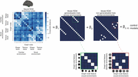
Neural analysis framework. To test whether MTL subregions distinguish generalizable and nongeneralizable information across environments, we performed an RSA. We first extracted neural data from the EC and computed cross-validated Mahalanobis distances (crossnobis distances) between all condition pairs. Unlike metrics that are not cross-validated, crossnobis distances can take on negative values when patterns contain noise. If the true distance is 0, this will result in distance estimates symmetrically distributed around 0 (Schütt et al., 2023). We then asked whether the resulting RDM exhibited a relative increase in neural similarity for stimuli at the starting location on each trial when transition information could be generalized across environments. The “gen. model” RDM (shown beside β₁) was formulated to capture cross-environment stimulus similarity for the generalizable feature dimension. In this case, each stimulus occupied the same graph node in both environments and therefore sequential transitions for this dimension could be generalized (shown in the green inset linked to the β₁ RDM). The “non-gen. model” RDM (shown beside β₂) was formulated to captured cross-environment stimulus similarity for the feature dimension that did not generalize. In this case, each stimulus was mapped to different node positions across graphs and therefore transitions for this feature dimension differed in the two environments (shown in the red inset linked to the β₂ RDM). These model RDMs were used as predictors in a multiple regression to explain the neural RDM. The regression procedure simultaneously controlled for a variety of other task factors that could plausibly influence the neural signal, including differences in accuracy between conditions and differences in visual information shown on screen. As a final step, we tested whether β₁ was significantly higher than β₂ as a representational marker distinguishing generalizable from nongeneralizable trials across environments. The same process was also applied to neural data extracted from the HPC.

In addition to the gen. and non-gen. model RDMs, we constructed control RDMs to account for other aspects of the neural signal (Fig. 3). These included models for condition differences in the environment, block type, animal cue, and individualized control RDMs for the number of on-screen stimulus matches during the response and feedback phases and condition differences in accuracy on the current and previous trial. Binary accuracy (the proportion of fully correct sequences reported) was used for the accuracy model RDMs, as opposed to transition accuracy (the proportion of correct transitions reported). This was because we were interested in testing whether neural signals distinguishing generalizable information had a functional connection to performance (transition accuracy) in the novel environment. Removing covariance from the neural signal associated with transition accuracy as a control RDM would be expected to eliminate a potential association between these variables. Using binary accuracy allowed us to control for overarching condition differences in accuracy while still retaining relevant covariation for neuro-behavioral tests. In addition to the control model described so far, we formulated control RDMs to account for various graph properties. These included model RDMs for the shortest bidirectional distance between nodes (link distance), the average bidirectional distance between nodes, the one-step bidirectional transitions within each environment–block context, and the node type (i.e., whether a node was a hub in the graph, an input to the hub or an output from the hub). The upper triangular portion of the neural and model RDMs was transformed into vectors and z-scored. The subsequent distance vectors were then entered into the following general linear model at each TR. Neural RDMs were computed using all trials (unless otherwise stated), and each TR here refers to a common timepoint across trials from the start of the planning phase:<mml:math display="block"><mml:mtable columnalign="right left" rowspacing=".5em" columnspacing="thickmathspace" displaystyle="true"><mml:mtr><mml:mtd><mml:mrow><mml:mi mathvariant="normal">Neural</mml:mi></mml:mrow><mml:mspace width=".1em"></mml:mspace><mml:mrow><mml:mi mathvariant="normal">DV</mml:mi></mml:mrow><mml:mo>=</mml:mo></mml:mtd><mml:mtd><mml:mspace width="0.25em"></mml:mspace><mml:msub><mml:mi>β</mml:mi><mml:mn>0</mml:mn></mml:msub><mml:mo>+</mml:mo><mml:mo stretchy="false">(</mml:mo><mml:mrow><mml:msub><mml:mi>β</mml:mi><mml:mn>1</mml:mn></mml:msub><mml:mo>×</mml:mo><mml:mrow><mml:mi mathvariant="normal">cued</mml:mi><mml:mspace width="0.25em"></mml:mspace></mml:mrow><mml:mspace width=".1em"></mml:mspace><mml:mrow><mml:mi mathvariant="normal">stimulu</mml:mi></mml:mrow><mml:msub><mml:mrow><mml:mi mathvariant="normal">s</mml:mi></mml:mrow><mml:mrow><mml:mrow><mml:mi mathvariant="normal">gen</mml:mi></mml:mrow></mml:mrow></mml:msub><mml:mspace width="0.25em"></mml:mspace><mml:mrow><mml:mi mathvariant="normal">DV</mml:mi></mml:mrow></mml:mrow><mml:mo stretchy="false">)</mml:mo></mml:mtd></mml:mtr><mml:mtr><mml:mtd></mml:mtd><mml:mtd><mml:mspace width="1em"></mml:mspace><mml:mo>+</mml:mo><mml:mspace width="0.25em"></mml:mspace><mml:mo stretchy="false">(</mml:mo><mml:mrow><mml:msub><mml:mi>β</mml:mi><mml:mn>2</mml:mn></mml:msub><mml:mo>×</mml:mo><mml:mrow><mml:mi mathvariant="normal">cued</mml:mi></mml:mrow><mml:mspace width=".1em"></mml:mspace><mml:mrow><mml:mi mathvariant="normal">stimulu</mml:mi></mml:mrow><mml:msub><mml:mrow><mml:mi mathvariant="normal">s</mml:mi></mml:mrow><mml:mrow><mml:mrow><mml:mi mathvariant="normal">non</mml:mi></mml:mrow><mml:mstyle displaystyle="false" scriptlevel="0"><mml:mtext>-</mml:mtext></mml:mstyle><mml:mrow><mml:mi mathvariant="normal">gen</mml:mi></mml:mrow></mml:mrow></mml:msub><mml:mspace width="0.25em"></mml:mspace><mml:mrow><mml:mi mathvariant="normal">DV</mml:mi></mml:mrow></mml:mrow><mml:mo stretchy="false">)</mml:mo></mml:mtd></mml:mtr><mml:mtr><mml:mtd></mml:mtd><mml:mtd><mml:mspace width="1em"></mml:mspace><mml:mo>+</mml:mo><mml:mo stretchy="false">(</mml:mo><mml:mrow><mml:msub><mml:mi>β</mml:mi><mml:mn>3</mml:mn></mml:msub><mml:mo>×</mml:mo><mml:mrow><mml:mi mathvariant="normal">environment</mml:mi><mml:mspace width="0.25em"></mml:mspace></mml:mrow><mml:mspace width=".1em"></mml:mspace><mml:mrow><mml:mi mathvariant="normal">DV</mml:mi></mml:mrow></mml:mrow><mml:mo stretchy="false">)</mml:mo><mml:mo>+</mml:mo><mml:mo stretchy="false">(</mml:mo><mml:mrow><mml:msub><mml:mi>β</mml:mi><mml:mn>4</mml:mn></mml:msub><mml:mo>×</mml:mo><mml:mrow><mml:mi mathvariant="normal">block</mml:mi></mml:mrow><mml:mspace width=".1em"></mml:mspace><mml:mrow><mml:mi mathvariant="normal">type</mml:mi></mml:mrow><mml:mspace width=".1em"></mml:mspace><mml:mrow><mml:mi mathvariant="normal">DV</mml:mi></mml:mrow></mml:mrow><mml:mo stretchy="false">)</mml:mo></mml:mtd></mml:mtr><mml:mtr><mml:mtd></mml:mtd><mml:mtd><mml:mspace width="1em"></mml:mspace><mml:mo>+</mml:mo><mml:mo stretchy="false">(</mml:mo><mml:mrow><mml:msub><mml:mi>β</mml:mi><mml:mn>5</mml:mn></mml:msub><mml:mo>×</mml:mo><mml:mrow><mml:mi mathvariant="normal">animal</mml:mi></mml:mrow><mml:mspace width=".1em"></mml:mspace><mml:mrow><mml:mi mathvariant="normal">cue</mml:mi></mml:mrow><mml:mspace width=".1em"></mml:mspace><mml:mrow><mml:mi mathvariant="normal">DV</mml:mi></mml:mrow></mml:mrow><mml:mo stretchy="false">)</mml:mo><mml:mo>+</mml:mo><mml:mo stretchy="false">(</mml:mo><mml:mrow><mml:msub><mml:mi>β</mml:mi><mml:mn>6</mml:mn></mml:msub><mml:mo>×</mml:mo><mml:mrow><mml:mi mathvariant="normal">link</mml:mi></mml:mrow><mml:mspace width=".1em"></mml:mspace><mml:mrow><mml:mi mathvariant="normal">distance</mml:mi><mml:mspace width="0.25em"></mml:mspace></mml:mrow><mml:mspace width=".1em"></mml:mspace><mml:mrow><mml:mi mathvariant="normal">DV</mml:mi></mml:mrow></mml:mrow><mml:mo stretchy="false">)</mml:mo></mml:mtd></mml:mtr><mml:mtr><mml:mtd></mml:mtd><mml:mtd><mml:mspace width="1em"></mml:mspace><mml:mo>+</mml:mo><mml:mspace width="0.25em"></mml:mspace><mml:mo stretchy="false">(</mml:mo><mml:msub><mml:mi>β</mml:mi><mml:mn>7</mml:mn></mml:msub><mml:mo>×</mml:mo><mml:mrow><mml:mi mathvariant="normal">average</mml:mi></mml:mrow><mml:mspace width=".1em"></mml:mspace><mml:mrow><mml:mi mathvariant="normal">node</mml:mi></mml:mrow><mml:mspace width=".1em"></mml:mspace><mml:mrow><mml:mi mathvariant="normal">distance</mml:mi></mml:mrow><mml:mspace width=".1em"></mml:mspace><mml:mrow><mml:mi mathvariant="normal">DV</mml:mi></mml:mrow><mml:mo stretchy="false">)</mml:mo></mml:mtd></mml:mtr><mml:mtr><mml:mtd></mml:mtd><mml:mtd><mml:mspace width="1em"></mml:mspace><mml:mo>+</mml:mo><mml:mo stretchy="false">(</mml:mo><mml:mrow><mml:msub><mml:mi>β</mml:mi><mml:mn>8</mml:mn></mml:msub><mml:mo>×</mml:mo><mml:mrow><mml:mi mathvariant="normal">context</mml:mi><mml:mspace width="0.25em"></mml:mspace></mml:mrow><mml:mspace width=".1em"></mml:mspace><mml:mrow><mml:mi mathvariant="normal">specific</mml:mi><mml:mspace width="0.25em"></mml:mspace></mml:mrow><mml:mspace width=".1em"></mml:mspace><mml:mrow><mml:mi mathvariant="normal">bidirectional</mml:mi></mml:mrow><mml:mspace width=".1em"></mml:mspace><mml:mrow><mml:mi mathvariant="normal">transitions</mml:mi></mml:mrow><mml:mspace width=".1em"></mml:mspace><mml:mrow><mml:mi mathvariant="normal">DV</mml:mi></mml:mrow></mml:mrow><mml:mo stretchy="false">)</mml:mo></mml:mtd></mml:mtr><mml:mtr><mml:mtd></mml:mtd><mml:mtd><mml:mspace width="1em"></mml:mspace><mml:mo>+</mml:mo><mml:mo stretchy="false">(</mml:mo><mml:mrow><mml:msub><mml:mi>β</mml:mi><mml:mn>9</mml:mn></mml:msub><mml:mo>×</mml:mo><mml:mrow><mml:mi mathvariant="normal">node</mml:mi></mml:mrow><mml:mspace width=".1em"></mml:mspace><mml:mrow><mml:mi mathvariant="normal">type</mml:mi></mml:mrow></mml:mrow><mml:mo stretchy="false">)</mml:mo><mml:mo>+</mml:mo><mml:mo stretchy="false">(</mml:mo><mml:mrow><mml:msub><mml:mi>β</mml:mi><mml:mn>10</mml:mn></mml:msub><mml:mo>×</mml:mo><mml:mrow><mml:mi mathvariant="normal">binary</mml:mi><mml:mspace width="0.25em"></mml:mspace></mml:mrow><mml:mspace width=".1em"></mml:mspace><mml:mrow><mml:mi mathvariant="normal">accurac</mml:mi></mml:mrow><mml:msub><mml:mrow><mml:mi mathvariant="normal">y</mml:mi></mml:mrow><mml:mrow><mml:mrow><mml:mi mathvariant="normal">trial</mml:mi><mml:mspace width="0.25em"></mml:mspace></mml:mrow><mml:mi>t</mml:mi></mml:mrow></mml:msub><mml:mspace width="0.25em"></mml:mspace><mml:mrow><mml:mi mathvariant="normal">DV</mml:mi></mml:mrow></mml:mrow><mml:mo stretchy="false">)</mml:mo></mml:mtd></mml:mtr><mml:mtr><mml:mtd></mml:mtd><mml:mtd><mml:mspace width="1em"></mml:mspace><mml:mo>+</mml:mo><mml:mo stretchy="false">(</mml:mo><mml:mrow><mml:msub><mml:mi>β</mml:mi><mml:mn>11</mml:mn></mml:msub><mml:mo>×</mml:mo><mml:mrow><mml:mi mathvariant="normal">binary</mml:mi></mml:mrow><mml:mspace width=".1em"></mml:mspace><mml:mrow><mml:mi mathvariant="normal">accurac</mml:mi></mml:mrow><mml:msub><mml:mrow><mml:mi mathvariant="normal">y</mml:mi></mml:mrow><mml:mrow><mml:mrow><mml:mi mathvariant="normal">trial</mml:mi></mml:mrow><mml:mspace width="0.25em"></mml:mspace><mml:mi>t</mml:mi><mml:mo>−</mml:mo><mml:mn>1</mml:mn></mml:mrow></mml:msub><mml:mspace width="0.25em"></mml:mspace><mml:mrow><mml:mi mathvariant="normal">DV</mml:mi></mml:mrow></mml:mrow><mml:mo stretchy="false">)</mml:mo></mml:mtd></mml:mtr><mml:mtr><mml:mtd></mml:mtd><mml:mtd><mml:mspace width="1em"></mml:mspace><mml:mo>+</mml:mo><mml:mo stretchy="false">(</mml:mo><mml:mrow><mml:msub><mml:mi>β</mml:mi><mml:mn>12</mml:mn></mml:msub><mml:mo>×</mml:mo><mml:mrow><mml:mi mathvariant="normal">visual</mml:mi></mml:mrow><mml:mspace width=".1em"></mml:mspace><mml:mrow><mml:mi mathvariant="normal">similarit</mml:mi></mml:mrow><mml:msub><mml:mrow><mml:mi mathvariant="normal">y</mml:mi></mml:mrow><mml:mrow><mml:mrow><mml:mi mathvariant="normal">rsp</mml:mi></mml:mrow><mml:mrow><mml:mo>.</mml:mo><mml:mspace width="0.25em"></mml:mspace><mml:mspace width="0.25em"></mml:mspace><mml:mi mathvariant="normal">phase</mml:mi></mml:mrow></mml:mrow></mml:msub><mml:mspace width="0.25em"></mml:mspace><mml:mrow><mml:mi mathvariant="normal">DV</mml:mi></mml:mrow></mml:mrow><mml:mo stretchy="false">)</mml:mo></mml:mtd></mml:mtr><mml:mtr><mml:mtd></mml:mtd><mml:mtd><mml:mspace width="1em"></mml:mspace><mml:mo>+</mml:mo><mml:mspace width="0.25em"></mml:mspace><mml:mo stretchy="false">(</mml:mo><mml:mrow><mml:msub><mml:mi>β</mml:mi><mml:mn>13</mml:mn></mml:msub><mml:mo>×</mml:mo><mml:mrow><mml:mi mathvariant="normal">visual</mml:mi></mml:mrow><mml:mspace width=".1em"></mml:mspace><mml:mrow><mml:mi mathvariant="normal">similarit</mml:mi></mml:mrow><mml:msub><mml:mrow><mml:mi mathvariant="normal">y</mml:mi></mml:mrow><mml:mrow><mml:mrow><mml:mi mathvariant="normal">feedback</mml:mi></mml:mrow></mml:mrow></mml:msub><mml:mspace width="0.25em"></mml:mspace><mml:mrow><mml:mi mathvariant="normal">DV</mml:mi></mml:mrow></mml:mrow><mml:mo stretchy="false">)</mml:mo><mml:mo>+</mml:mo><mml:mspace width="0.25em"></mml:mspace><mml:mi>ε</mml:mi><mml:mo>.</mml:mo></mml:mtd></mml:mtr></mml:mtable></mml:math>NeuralDV=β0+(β1×cuedstimulusgenDV)+(β2×cuedstimulusnon-genDV)+(β3×environmentDV)+(β4×blocktypeDV)+(β5×animalcueDV)+(β6×linkdistanceDV)+(β7×averagenodedistanceDV)+(β8×contextspecificbidirectionaltransitionsDV)+(β9×nodetype)+(β10×binaryaccuracytrialtDV)+(β11×binaryaccuracytrialt−1DV)+(β12×visualsimilarityrsp.phaseDV)+(β13×visualsimilarityfeedbackDV)+ε.

View larger version:

• In this window
• In a new window

• Download as PowerPoint Slide

Figure 3.

Control RDMs. A, RDMs capturing condition differences for the main task variables. These include environment (novel vs familiar), block type (report shape sequences vs report texture sequences), and animal cue. B, RDMs capturing condition differences based on the graph structure. These include model RDMs for the average bidirectional distance between nodes, the shortest bidirectional distance between nodes (i.e., the link distance), the node type (i.e., whether a node was a hub in the graph, an input to the hub or an output from the hub), and one-step bidirectional transitions within each environment–block context. C, Example model RDMs capturing differences in binary accuracy between conditions for an individual participant. This measure is the difference in proportion of fully correct sequence entries between two conditions. Model RDMs capture differences in accuracy based on the current and previous trial, respectively. D, Example model RDMs capturing how often stimuli presented on-screen match between conditions for an individual participant. Model RDMs capture such visual matches during the response and feedback phases, respectively. A–D, Lighter colors indicate a relative increase in similarity for all RDMs.

The resulting <mml:math display="inline"><mml:msub><mml:mi>β</mml:mi><mml:mn>1</mml:mn></mml:msub></mml:math>β1 and <mml:math display="inline"><mml:msub><mml:mi>β</mml:mi><mml:mn>2</mml:mn></mml:msub></mml:math>β2 coefficients were averaged from +3.75 to 15 s following cue onset. To test whether representational similarity across environments was significantly above zero in each ROI, we compared the resulting <mml:math display="inline"><mml:msub><mml:mi>β</mml:mi><mml:mn>1</mml:mn></mml:msub></mml:math>β1 and <mml:math display="inline"><mml:msub><mml:mi>β</mml:mi><mml:mn>2</mml:mn></mml:msub></mml:math>β2 coefficients against zero using two-sided permutation tests. To assess whether MTL subregions were distinguishing shared and unshared elements across environments, we tested whether the <mml:math display="inline"><mml:msub><mml:mi>β</mml:mi><mml:mn>1</mml:mn></mml:msub></mml:math>β1 and <mml:math display="inline"><mml:msub><mml:mi>β</mml:mi><mml:mn>2</mml:mn></mml:msub></mml:math>β2 coefficients were significantly different from each other using two-sided paired permutation tests. Condition labels for the coefficients were randomly swapped over 10,000 iterations, and the mean coefficient difference between conditions was computed to generate the null distribution. If the true sample difference fell within the 95th percentile of the null distribution, neural similarity was deemed significantly different in the generalizable and nongeneralizable blocks of the novel environment. To test for a neural distinction during early exposure to the novel environment, we repeated the analysis pipeline but restricted the analysis to only use trials from the first half of scanning in the novel environment (Trials 1–80 of a possible 160) to compute crossnobis distance estimates. Coefficient tests against 0 were corrected for multiple comparisons using the Benjamini–Hochberg correction (Benjamini and Hochberg, 1995). Tests of the difference between generalization coefficients (<mml:math display="inline"><mml:msub><mml:mi>β</mml:mi><mml:mn>1</mml:mn></mml:msub></mml:math>β1 vs <mml:math display="inline"><mml:msub><mml:mi>β</mml:mi><mml:mn>2</mml:mn></mml:msub></mml:math>β2 ) were uncorrected because they were derived from prior theoretical and empirical work (Behrens et al., 2018; Koolschijn et al., 2019; Baram et al., 2021; Glitz et al., 2022; Whittington et al., 2022).

Neural signaling of generalizable transition information

To test whether the neural distinction between generalizable and nongeneralizable feature dimensions extended past the cued staring location in each graph, we repeated the previous analysis but included three additional model RDMs for one-step forward transitions (Fig. 4). The models assumed that when an animal cue was shown in the novel environment, the next feature would be reactivated. Like the previous section, we used cross-environment similarity to isolate specific feature transitions (e.g., a specific shape independent from the texture and animal cue). Within-environment comparisons can be used to assess transition information in the neural signal but only for combinations of animal cues/features. Two model RDMs were used to isolate one-step feature transitions in the generalizable blocks and nongeneralizable blocks in response to each cue in the novel environment. A final model RDM was used to isolate feature transitions in the nongeneralizable blocks based on the old transition structure from the familiar environment, which was no longer relevant. The resulting coefficients were compared in a 3 × 2 repeated-measure ANOVA, with factors of transition model (gen. forward vs non-gen. forward vs non-gen. irrel. forward) and ROI (EC. vs HPC). In addition to performing this analysis using data from the planning phase (+3.75 to 15 s following cue onset), we performed follow-up tests that examined possible differences between forward transition models during the response phase (+15 to +20 s following cue onset) and transient differences across time using cluster-based permutation testing (+3.75 to +20 s following cue onset; Maris and Oostenveld, 2007).

View larger version:

• In this window
• In a new window

• Download as PowerPoint Slide

Figure 4.

Model RDMs for one-step forward transitions. A, Example graphs for an individual participant, as shown in the main text. B, Example forward transition models. The main aim of the models is to test the idea that when an animal cue is shown in the novel environment, the stimulus at the next node in the graph gets activated. This activation is then expected to increase the neural similarity between the current condition in the novel environment and the condition in the familiar environment that began with that activated feature. i, The model RDM on the left captures one-step forward transitions for the generalizable blocks of the novel environment. For example, seeing an elephant cue in the novel environment during a shape block (the circle node) would lead to the activation of the triangle as the next node, increasing the similarity with lemur trials in the familiar environment where the triangle was cued. ii, The model RDM in the middle captures one-step forward transitions for the nongeneralizable blocks. For example, seeing an elephant cue in the novel environment during a texture block (the node with the dotted-column texture) would lead to the activation of the horizontal line texture as the next node, increasing the similarity with zebra trials in the familiar environment where that texture was cued. iii, The model RDM on the right captures one-step forward transitions in the nongeneralizable blocks, based on the irrelevant graph structure from the familiar environment. For example, seeing an elephant cue in the novel environment during a texture block (the node with the dotted-column texture), it would be as if the participant was in the top right node of the familiar environment (a node which also has the dotted-column texture). Planning one step from this point would lead to activation of the wave texture, increasing the similarity with lemur trials from the familiar environment.

Exploratory regions of interest

To assess whether regions outside the MTL distinguished the generalizable and nongeneralizable dimensions, we repeated the analysis outlined above, Neural signaling of generalizable feature information, for several exploratory ROIs. These included the medial orbitofrontal cortex, rostral anterior cingulate cortex, dorsolateral prefrontal cortex, inferior parietal cortex, and precuneus. Exploratory regions were selected based on past research implicating them in graph-like representations or the generalization of latent task structure (Schuck et al., 2016; Park et al., 2020; Vaidya et al., 2021; Baram et al., 2024). The resulting coefficient magnitudes were analyzed within a 2 × 7 repeated-measures ANOVA, with factors of model (gen. vs non-gen.) and ROI (the five exploratory regions, plus EC and HPC).

Neural signaling and performance

Spearman correlations were used to test whether neural signals identified in the EC were correlated with performance in the novel environment. The variables used in the correlations were the difference between the gen. and non-gen. model coefficients (<mml:math display="inline"><mml:msub><mml:mi>β</mml:mi><mml:mn>1</mml:mn></mml:msub></mml:math>β1 and <mml:math display="inline"><mml:msub><mml:mi>β</mml:mi><mml:mn>2</mml:mn></mml:msub></mml:math>β2 ) in EC based on Trials 1–80 in the novel environment (1–80) and the difference in performance on those same trials between generalizable or nongeneralizable blocks. Follow-up tests examined whether the neural difference correlated with performance in the generalizable or nongeneralizable blocks individually. A Williams test was used to examine whether the correlation strength was significantly higher for the neuro-behavioral correlation involving generalizable blocks compared with the correlation involving nongeneralizable blocks. A second Williams test was used to examine whether the correlation strength was significantly higher in the EC than in the HPC. The Benjamini–Hochberg procedure (Benjamini and Hochberg, 1995) was used to correct for equivalent correlation tests within the main (EC and HPC) and exploratory (medial orbitofrontal cortex, rostral anterior cingulate cortex, dorsolateral prefrontal cortex, inferior parietal cortex, and precuneus) ROI families.